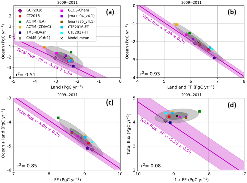
Figure 4.

Synthesis of globally integrated fluxes for the 2009–2011 period, in PgC yr⁻¹. Each inversion is represented by a square and the model mean by a × symbol. The GCP2016 estimates are a pink diamond, which is sometimes hard to see because it is superimposed in each panel by the gray CAMS point. We have adjusted the GCP2016 ocean and land flux estimates by the riverine flux of carbon from land to ocean to atmosphere (0.45 PgC yr⁻¹; Jacobson et al., 2007; Le Quéré et al., 2018), decreasing the ocean sink and increasing the land sink. The magenta line and light-pink shaded area show the corresponding mass balance estimates from GCP2016. In each panel the line and equation shown represent the sum of the x and y variables, and thus the line has a slope of −1, and any deviation perpendicular to the line indicates disagreement on the sum. Here we use the total flux which by mass balance is the whole-atmosphere growth rate (see text), and for panels (a) and (d), the total flux – FF line also equals O + L, while for panels (b) and (c), the total flux line equals O + L + FF. Ellipses denote the variability around the model means of 1σ (darker gray) and 2σ (lighter gray). (a) Ocean versus land; (b) ocean versus land + FF; (c) ocean + land versus FF; (d) total flux versus − 1 × FF.