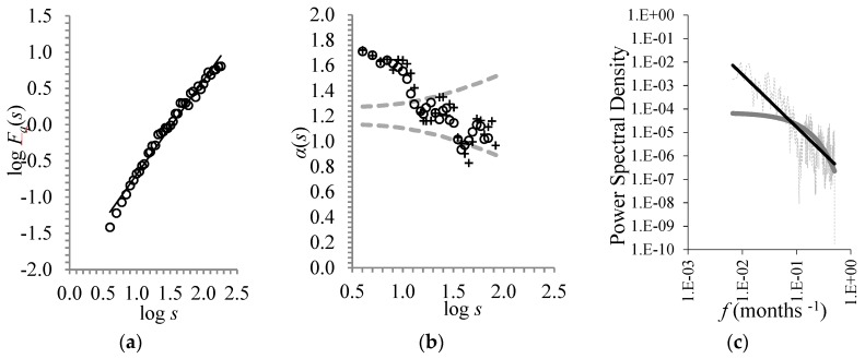
Figure 2.

(a) The root-mean-square fluctuation function F_d(s) of the CST time-series as a function of time scale s (in years). The corresponding best fit equation is y = 1.30x − 1.99 (R² = 0.98). (b) The variability of the power-law exponent expressed as local slopes of the logF_d(s) vs. log s calculated within a window of 12 points (circles) and 10 points (crosses). The dashed grey line represents the 2s_a intervals around the local slopes with an average value of $\overline{a}$ = 1.2. (c) The power spectral density as a function of frequency (a) (dashed gray line) with a power-law fit (black line) (y = 1·10⁻⁷·x^−2.24 with R² = 0.56) and the exponential fit (grey line) (y = 7·10⁻⁵·e^−11.5x with R² = 0.39).