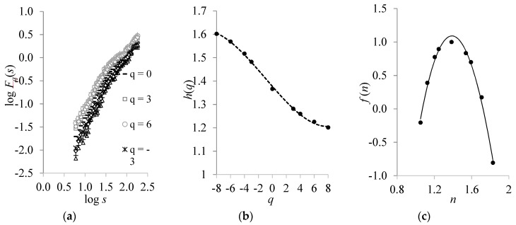
Figure 5.
As in Figure 3, but for the detrended and deseasonalized CST time-series. (a) In (b), the empirical curve (dots) was fitted by the polynomial h(q) = 1·10−4q3 + 4·10−4q2 − 0.03q + 1.38, with R² = 1.00. In (c), the empirical curve (dots) was fitted with f(n) = 1.61n3 − 17.06n2 + 38.06n − 23.18, with R² = 0.99.

