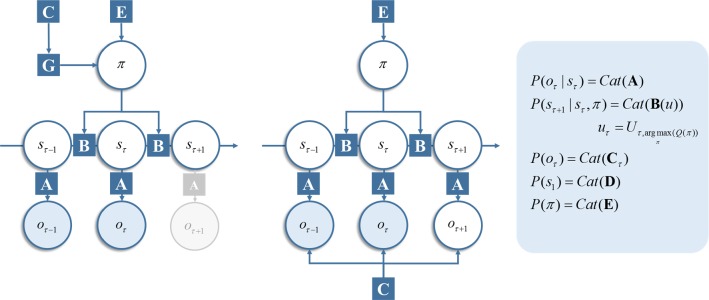
Fig. 1.

Markov decision process. This shows the basic structure of the discrete state-space generative model used in this paper, assuming the current time is t = τ. The factor graph on the left is the generative model we have used in previous work. Importantly, the prior belief about observations only enters this graph through the expected free energy, $G$ (see main text), which enters the prior over policies. Policies index alternative trajectories, or sequences, of actions. In this sense, they are not time dependent, as each policy determines a sequence of actions for all time-points. Conversely, the actions (u) are time dependent. U is an array that specifies an action for each time step (rows) and each policy (columns). The selected action therefore depends upon the most likely policy and the action that policy implies for that time step. Action selection is technically not part of the generative model, as it relies upon the posterior distribution Q (please see main text for details), obtained by inverting the model. This is an important, aspect of active inference, as it underwrites the way in which the system performing inference may change the process generating its observed data. The grey region of this graph indicates that the observation at the next time step is not yet available, so cannot yet be incorporated into the graph. The right factor graph is the new version of the generative model considered in this paper. This generative model does not require an expected free energy, and the prior over outcomes enters the model directly as a constraint on outcomes. This also shows a time dependence, as future outcomes are treated as unobserved latent variables (indicated by an unfilled circle). Observed variables are shown as filled circles in both graphs and unobserved variables as unfilled circles. Factors of the generative model (i.e. conditional probability distributions and prior probabilities) are shown as squares. These squares are connected to those circles containing variables that participate in the same factor. Please refer to the main text and Table 2 for a description of the variables. In the panel on the right, the definitions are given for each of the factors in blue squares. Here, Cat refers to the categorical distribution (color figure online)