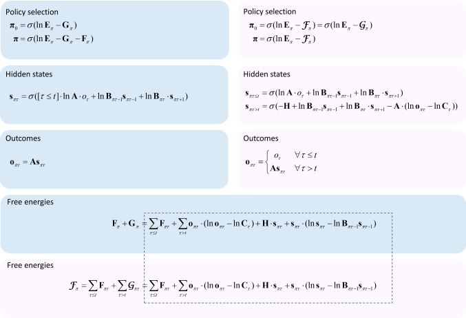
Fig. 3.

Belief update equations. The blue panels show the update equations using the standard variational approach. The pink panels show the update equations when the generalised free energy is used. The equations in this figure show the fixed points for the sufficient statistics of each variational distribution. These are calculated as in the main text by finding the minima of each of the free energy functionals. As such, updating the variational distributions (left-hand side of each equation) to their fixed points (right-hand side of each equation) following each new observation minimises the corresponding free energy. The dotted outline indicates the correspondence between the generalised free energy and the sum of the variational and expected free energies, and therefore the equivalence of the form of the posteriors over policies. However, it should be remembered that the variables within these equations are not identical, as the update equations demonstrate. See Table 2 for the definitions of the variables as they appear here. The equations used here are discrete updates. A more biologically plausible (gradient ascent) scheme is used in the simulations. These simply replace the updates with differential equations that have stationary points corresponding to the variational solutions above. Because the belief updates specified in Fig. 3 take each belief distribution to its free energy minimum, the belief updates and corresponding policy choices necessarily minimise free energy. In the update equations shown here, o_τ is treated as a binary vector with one in the element corresponding to the observed data, and zero for all other elements. This ensures consistency with the linear algebraic expression of the update equations (color figure online)