Fig. 4.

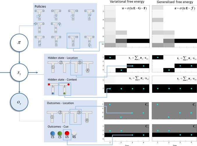
T-maze simulation. The left part of this figure shows the structure of the generative model used to illustrate the behavioural consequences of each set of update equations. We have previously used this generative model to address exploration and exploitation in two-step tasks; further details of which can be found in Friston et al. (2015). In brief, an agent can find itself in one of four different locations and can move among these locations. Locations 2 and 3 are absorbing states, so the agent is not able to leave these locations once they have been visited. The initial location is always 1. Policies define the possible sequences of movements the agent can take throughout the trial. For all ten available policies, after the second action, the agent stays where it is. There are two possible contexts: the unconditioned stimulus (US) may be in the left or right arm of the maze. The context and location together give rise to observable outcomes. The first of these is the location, which is obtained through an identity mapping from the hidden state representing location. The second outcome is the cue that is observed. In location 1, a conditioned stimulus (CS) is observed, but there is a 50% chance of observing blue or green, regardless of the context, so this is uninformative (and ambiguous). Location 4 deterministically generates a CS based on the context, so visiting this location resolves uncertainty about the location of the US. The US observation is probabilistically dependent on the context. It is observed with a 90% chance in the left arm in context 1 and a 90% chance in the right arm in context 2. The right part of this figure compares an agent that minimises its variational free energy (under the prior belief that it will select policies with a low expected free energy) with an agent that minimises its generalised free energy. The upper plots show the posterior beliefs about policies, where darker shades indicate more probable policies. Below these, the posterior beliefs about states (location and context) are shown, with blue dots superimposed to show the true states used to generate the data. The lower plots show the prior beliefs about outcomes (i.e. preferences), and the true outcomes (blue dots) the agent encountered. Note that a US is preferred to either CS, both of which are preferable to no stimulus (NS). Outcomes are observed at each time step, depending upon actions selected at the previous step. The time steps shown here align with the sequence of events during a trial, such that a new outcome is available at each step. Actions induce transitions from one time step to the next (color figure online)