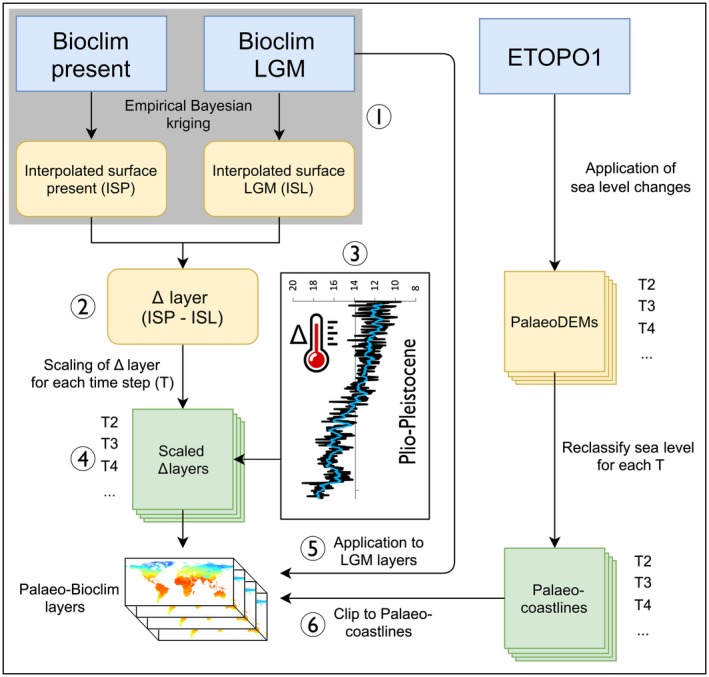
Figure 1.

Flowchart for generating interpolated palaeo‐bioclim layers (Oscillayers). Step 1: Empirical Bayesian kriging interpolation of each variable for the present and the Last Glacial Maximum (LGM). Step 2: Computation of the Δ layers. Step 3: Calculation of surface temperature (Ts) differences between the LGM and proceeding time periods as derived from the isotope record for each time step (T). Step 4: Scaling the Δ layers relative to those differences of Step 3. Step 5: Application of the scaled Δ layers to the LGM variables for calibration. Step 6: Clipping each layer with the corresponding palaeo‐coastlines, as derived from reclassified digital elevation models (DEMs), to obtain the calibrated palaeo‐bioclim layers of each time period (Oscillayers) [Colour figure can be viewed at https://www.wileyonlinelibrary.com]