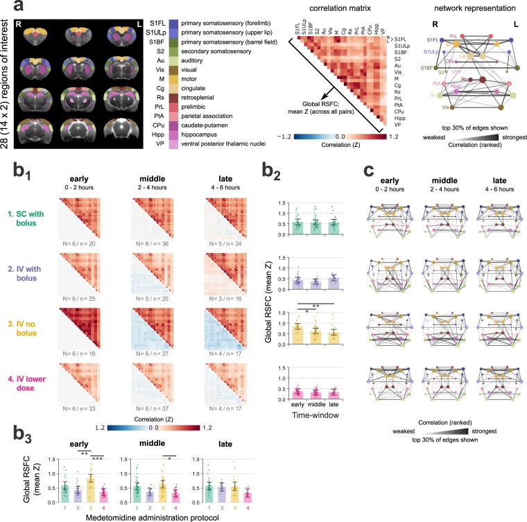
Figure 5.
Resting state functional connectivity (RSFC). (a) To calculate pair-wise RSFC, 28 regions-of-interest (ROIs) were defined based on the Paxinos-Watson rat brain atlas—14 on each hemisphere. Pearson’s correlations were calculated between the BOLD time courses of all unique ROI pairs and transformed into Fisher’s Z-scores. A pair-wise correlation matrix is shown for one example RS-fMRI run; the mean correlation (Z-score) across all ROI pairs constitutes the global RSFC. The matrix is also represented as a weighted network graph, with the ROIs as nodes and their pairs as edges. For visualization clarity, only the strongest 30% of edges are shown; edge thickness and opacity scale linearly with the relative rank of the correlation value (the highest Z-score corresponds to the thickest edge); node radius scales with the weighted degree (weighted sum of edges passing through the node). (b) The 295 RS-fMRI runs are split into twelve groups according to the applied medetomidine protocol and the time-window since the start of medetomidine administration (early: 0–2 h; middle: 2–4 h; late: 4–6 h). (b1) For each group, the upper triangular matrix represents the mean (across runs) pair-wise correlation, while the lower triangular matrix shows the change in correlation compared to each protocol’s early period. N: number of rats; n: number of fMRI runs. In (b2) global RSFC values are plotted across time-windows for each of the medetomidine protocols, while in (b3) they are plotted across medetomidine protocols for each of the time-windows. Dots represent single run values, bars show the estimated Least Squares Means, while error margins correspond to the estimated 95% confidence intervals. Asterisks indicate the significance of pair-wise t-tests, after adjusting for multiple comparisons (p < 0.05: *, p < 0.01: **, p < 0.001: ***). Global RSFC time courses for individual rats are provided in Supplementary Fig. S7b. A complete list of Least Square Means, confidence intervals and pair-wise comparisons can be found in Supplementary Tables S10 and S12. (c) The mean correlation matrices (upper triangles of (b1)) are also visualized as network graphs, similarly to the example graph in (a).

