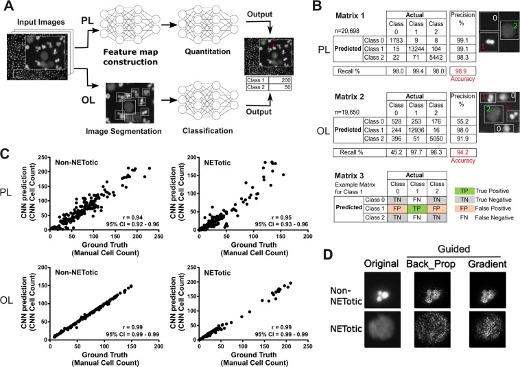
Figure 1.
(A) The first panel represents one field (672 × 512 pixels of a 16-bit image) out of 36 fields in a typical image; the inset contains nuclei with the annotations 1 or 2 corresponding to non-NETotic and NETotic nuclei, respectively. The annotations were generated manually using ImageJ. The pixel-level (PL) classifier was trained by scanning the whole image (a total of 4032 × 3072 pixels) in 32 × 32-pixel patches and classifying each patch as a class 1 or 2 using the annotations found on the image. The object-level (OL) classifier uses drawn bounding boxes of variable dimensions around all objects identified in the image and uses the object in the bounding box as training data. (B) Confusion matrices were used to evaluate model performance on the holdout dataset excluding the training dataset. The n numbers represent the holdout dataset only. The numbers in red denote model accuracy, which is the percentage of total correct predictions by the CNN. Recall is the number of true positives divided by true positive + false negative or the fraction of actual true positive predictions identified correctly. Precision is the number of true positive values divided by true positive + false positive or the fraction of positive identifications that were actually correct. An example of what would constitute true positive, true negative, false positive and false negative for class 1 is shown in matrix 3. Matrices 1 and 2 represent confusion matrices for PL and OL respectively. The nuclei images adjacent to the matrices indicate which nuclei were labeled as class 0, 1 or 2 by the two different CNN. The major difference in training of the CNNs is the class 0 category. (C) Pearson’s correlation coefficient (r) was used to compare the quantification of PL and OL (CNN prediction) to that performed manually (ground truth). A total of 186 and 161 images containing hundreds of cells were quantified by PL and OL, respectively, with a confidence interval of 95%, p < 0.0001 for all obtained R values. Each dot represents an image that was counted manually and by a CNN for the total number of Non-NETotic (graphs on the left), and NETotic cells (graphs on the right) in an image. (D) Guided backpropagation as well as gradient-weighted class activation mapping were used to generate saliency maps evaluating the relative contributions of each pixel to the CNN’s prediction. The brighter a pixel appears on this map, the more salient it is in identifying the phenotype and the more value it has in determining the CNN’s prediction.

