Figure - PMC

Skip to main content

An official website of the United States government

Here's how you know

Here's how you know

Official websites use .gov
A .gov website belongs to an official government organization in the United States.

Secure .gov websites use HTTPS
A lock ( ) or https:// means you've safely connected to the .gov website. Share sensitive information only on official, secure websites.

View full-text article in PMC

. 2019 Nov 19;9:16324. doi: 10.1038/s41598-019-51974-4

Search in PMC
Search in PubMed
View in NLM Catalog
Add to search

© The Author(s) 2019

Open Access This article is licensed under a Creative Commons Attribution 4.0 International License, which permits use, sharing, adaptation, distribution and reproduction in any medium or format, as long as you give appropriate credit to the original author(s) and the source, provide a link to the Creative Commons license, and indicate if changes were made. The images or other third party material in this article are included in the article’s Creative Commons license, unless indicated otherwise in a credit line to the material. If material is not included in the article’s Creative Commons license and your intended use is not permitted by statutory regulation or exceeds the permitted use, you will need to obtain permission directly from the copyright holder. To view a copy of this license, visit http://creativecommons.org/licenses/by/4.0/.

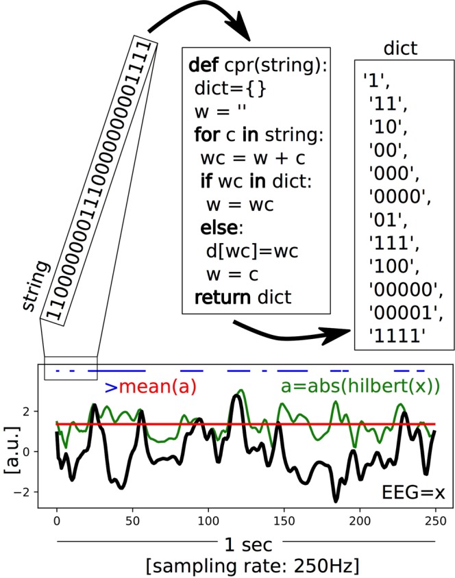
PMC Copyright notice

Schematic of the LZs computation. An example EEG signal with a sampling rate of 250 Hz and a length of 1 sec is shown in black (x). The mean (red) of the absolute value of its analytic signal (green, a) is used to binarize the signal (blue). The encoding step of the Lempel-Ziv algorithm is then applied to the first 25 entries of that binarized signal (in this illustration), creating a dictionary of the unique subsequences, which is then normalized by dividing the raw value by those obtained for the same randomly shuffled binary sequence. This provides a value between 0–1 that quantifies the temporal diversity of the EEG signal (LZs).