Figure 1.

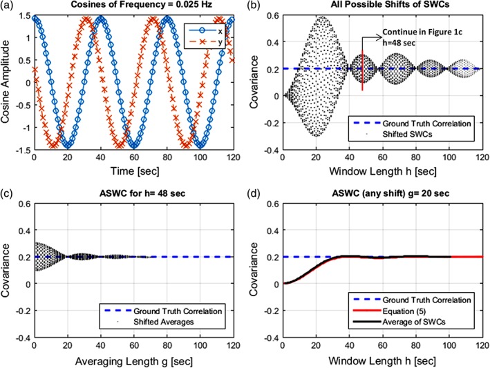
Averaging of the cosine model for a simulated correlation of 0.2. (a) The two cosines at the upper left plot were generated assuming a TR = 1 s, a frequency of f = 0.025 Hz and a phase difference given by θ = arccos(0.2). (b) Sliding window correlations (SWCs) were estimated at all possible shifts of one TR and for SWC lengths from 2 to 120 s. For a given window length, the SWC value depends on the time shift. SWCs for all time shifts are plotted on the upper right figure using small black dots. In this example, following the recommended SWC length (Leonardi & Van De Ville, 2015) will result in f_min = 0.025 Hz and h_min ≥ 1/f_min = 40 s. However, this figure shows that artifacts are still strong around approximately h = {50, 70, ⋯}. (c) The bottom left plot shows the effect of averaging for the window length h = 48 s, point where the stronger artifacts occur for that lobe. Spurious variability of SWCs disappears at the averaging length g =1/2f = 20 s. (d) the bottom right plot shows the resulting SWC value (black line) as a function of h at averaging length g = 20 s. The SWC values are independent of the time shift selected. For comparison, the asymptotic averaging result g → ∞ obtained in quation 5 is displayed in red. The two average settings g = 1/2f and g → ∞ lead to the same result [Color figure can be viewed at http://wileyonlinelibrary.com]