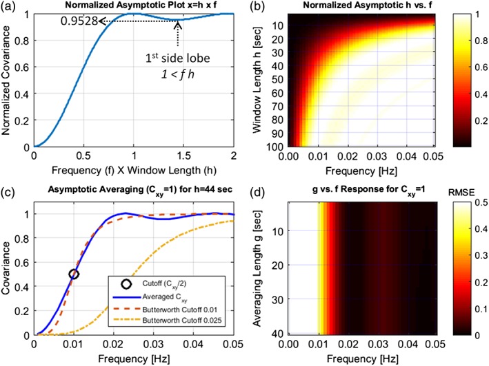
Figure 2.

Asymptotic response of ASWCs. (a) The left top plot displays the shape of asymptote (5) described by (1 − sinc²(x)) for the factor x = fh, where f is the frequency and h is the window length. (b) The right top plot illustrates the deleterious effects (perfect covariance estimation (${\overline{C}}_{\mathit{xy}}=1$) is indicated by white areas) predicted by (5) on covariance estimation for a range of values of f and h. This result indicates that low frequencies and low window lengths (dark red areas) must be avoided as they result in the largest deviation from ground truth. (c) The bottom left panel features a 15 min simulation using two identical cosines with ${\overline{C}}_{\mathit{xy}}=1$ for the same window length of 44 s but varying frequency. Since h = 44 s the cutoff frequency estimated by (6) is 0.01 Hz which is indicated by the circle drawn in the plot. The plot also shows how the filter compares to second order Butterworth filters using cutoffs of 0.01 Hz and 0.025 Hz. (d) The bottom right plot shows the root mean square error (RMSE) (averaged over 15 min) after setting h = 44 s for different frequencies and averaging lengths. The largest observed RMSE was 1.27, but fitting the color range to this value left obscured other smaller errors; hence, this plot was instead scaled to the (0, 0.5) range. The figure clearly shows the cut‐off 0.5 at 0.01 Hz, an observation that does not change with the averaging length [Color figure can be viewed at http://wileyonlinelibrary.com]