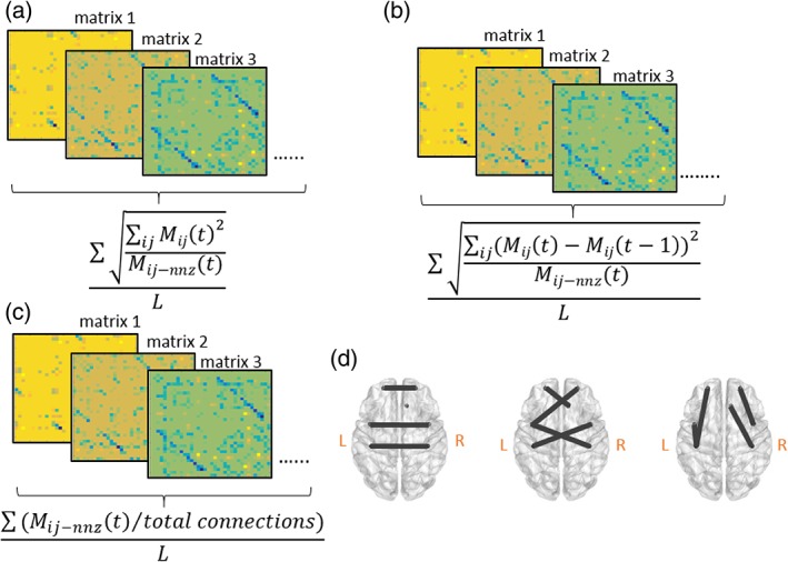
Figure 1.

(a) NP calculates the average connectivity strength across windows. (b) Density (DEN) computes how dense the existing connections are across windows. (c) NV) estimates the average global connectivity changes between two adjacent windows across time. (d) FOCcs, (e) FOCcns, and (f) FOCw measure the average connectivity changes in interhemispheric, cross‐hemispheric, and intrahemispheric connections between two adjacent windows across time, respectively. These features are illustrated in a graph fashion as the mathematical definitions are similar to (c) (details in Table 4). M _ij (t) is the i‐by‐j inverse covariance matrix containing every element at time t, M _ij (t‐1) is the i‐by‐j inverse covariance matrix containing every element at time t‐1. M _ij‐nnz (t) is the i‐by‐j inverse covariance matrix containing nonzero values at time t. L represents the total number of windowed matrices [Color figure can be viewed at http://wileyonlinelibrary.com]