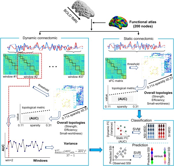
Figure 1.

A schematic illustration of the analysis approach. The preprocessed resting‐state BOLD fMRI time series are extracted using a functional atlas with 200 nodes. Static connectomic is constructed using a full‐length time series (230 TRs, 460 s) for each pair of two nodes. The topological properties (i.e., network strength, network efficiency, small‐worldness, and nodal efficiency) are calculated on series sparsity thresholded (0.11 ≤ sparsity ≤ 0.31) weighted matrices for each participant. The area under curve (AUC) of each topological property is computed for subsequent statistical analysis. Dynamic connectomic is constructed using a sliding‐window analysis with sliding‐window length of 50 TRs (100 s), and shifted with a step size of 5 TRs (10 s). The topological properties (i.e., network strength, network efficiency, small‐worldness, and nodal efficiency) are calculated on series sparsity thresholded (0.11 ≤ sparsity ≤ 0.31) weighted matrices in each sliding‐window for each participant. The AUC of each network property is computed for each sliding‐window. The variance of the AUC is then computed across 37 sliding‐windows for temporal variability of dynamic connectomic for subsequent statistical analysis. The overall topologies of both static and dynamic connectomics are used as features to distinguish the SI group from the NSI group using support vector machine (SVM) and to predict the severity of SI group using support vector regression (SVR) [Color figure can be viewed at http://wileyonlinelibrary.com]