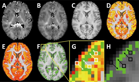
Figure 1.

Steps for processing gray matter based spatial statistics. (A) ICVF map. (B) Normalized ICVF map. (C) 3D T1‐weighted image. (D) Cortical tissue probability map. (E) Population mean cortical tissue probability map. (F) Skeletonized cortical map overlaid on a template. (H) Illustration of the region contained in the yellow square in F. The cortical probability map from D is transformed into the template space. Once aligned, the cortical voxels near the skeleton (shown in green) are identified (white squares). Data from these voxels are then projected onto the group skeleton for comparison (white arrows). (H) After aligning the ICVF map in A to the template, ICVF data from the voxels identified in G are projected onto the skeleton. This process is repeated for the other diffusion parameter maps. [Color figure can be viewed at http://wileyonlinelibrary.com]