Figure 1.

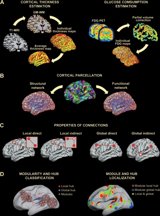
Analysis pipeline followed in this study. A. Cortical thickness estimation (left panel). T1‐MR images were segmented with Freesurfer to obtain individual cortical thickness maps that were further averaged to establish the cortical parcellation scheme. Cortical glucose consumption estimation (right panel). Partial volume effects were corrected on individual FDG‐PET cerebral images to obtain glucose consumption maps. B. Cortical parcellation. By applying a backtracking algorithm [Romero‐Garcia et al., 2012], the cortical surface was divided into 599 regions (with a surface area of 250 mm² each). Structural and functional cortical networks were based on thickness and glucose consumption, respectively, and adjacency matrices were obtained from this cortical scheme. C. Properties of connections. We calculated separately the influence of different structural connections (local direct, local indirect, global direct, and global indirect) on F‐S coupling for all network nodes, hubs (based on node degree and betweenness), and cortical regions grouped into modules. D. Left panel. Schematic representation of different types of hubs (local and global) and network modules (classification criteria are detailed in Materials and Methods). Right panel. Example of regional distribution of modular hubs in cortical networks. The color scale represents the proportion of sparsities for one specific region that reached the hub criterion.