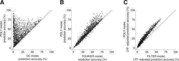
Figure 4.

Modeling LFF with polynomials maximizes prediction accuracy. In these graphs we compare different strategies for LFF compensation (Table I). For each graph, we selected voxels with a minimum SNR of 10 under either of the models being compared. Each point in a graph represents prediction accuracy for a single voxel. (A) DC vs. POLY. The x‐ and y‐axes indicate prediction accuracy under the DC and POLY models, respectively. There was a large increase in accuracy under the POLY model compared to the DC model (n = 1904; median increase 14.8%; P < 0.001). This indicates that ignoring LFF resulted in model fits with poor generalizability, and that a substantial amount of LFF exists in the time‐series data. Some voxels exhibited very large increases in prediction accuracy; in these cases, the contribution of LFF to variance in the time‐series data is much larger than the contribution of stimulus effects. (B) FOURIER vs. POLY. The x‐ and y‐axes indicate the prediction accuracy under the FOURIER and POLY models, respectively. There was a small increase in accuracy under the POLY model compared to the FOURIER model (n = 1,971; median increase 2.3%; P < 0.001). This indicates polynomials more accurately characterized LFF compared to Fourier basis functions in this data set. (C) FILTER vs. POLY. The x‐ and y‐axes indicate the LFF‐adjusted prediction accuracy under the FILTER and POLY models, respectively. There was a large increase in accuracy under the POLY model compared to the FILTER model (n = 1,880; median increase 6.5%; P < 0.001). This indicates that stimulus effects were better characterized when polynomials were used to model LFF compared to when the time‐series data were high‐pass filtered to remove LFF.