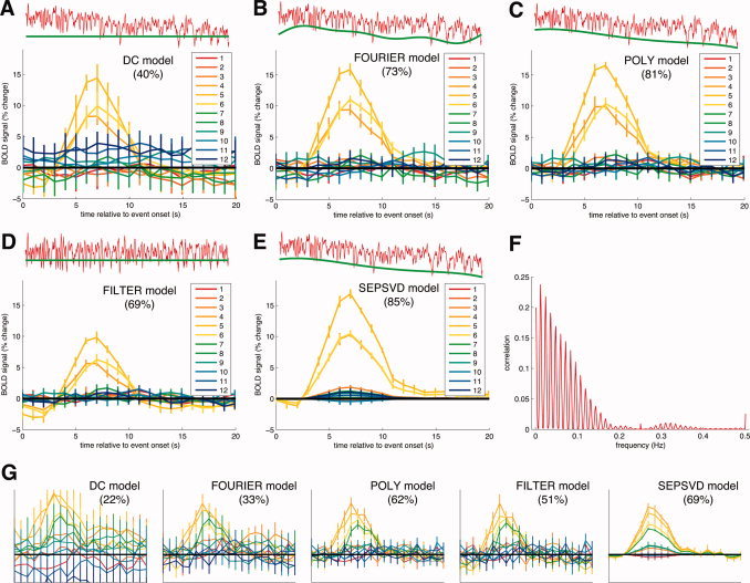
Figure 8.

Comparison of data models for two typical voxels in occipital cortex. Panels A–F depict one voxel, and panel G depicts a second voxel. In panels A–E and G, the main axes show HDR estimates for the 12 event types. The x‐axis indicates time relative to event onset; the y‐axis indicates percent BOLD change. A thick black horizontal line indicates zero percent BOLD change. Error bars indicate ±1 SE (jackknife procedure). Indicated in parentheses is the LFF‐adjusted prediction accuracy, which is calculated via 10‐fold cross‐validation. The inset axes above the main axes depict the time‐series data (red line) and nuisance effects (green line). (A) DC model. This model ignores LFF and uses only a constant term to characterize the baseline signal level. Under this model, HDR estimates were very noisy and prediction accuracy was poor. (B) FOURIER model. This model uses a constant term and Fourier basis functions with 1, 2, and 3 cycles to model LFF. Compared to the DC model, HDR estimates were less noisy and prediction accuracy was better. Note that the nuisance effects poorly track the time‐series data at the beginning and end of the time‐series. (C) POLY model. This model uses polynomials of degrees 0 through 4 to model LFF. Compared to the FOURIER model, HDR estimates were slightly less noisy and prediction accuracy was better. Notice the nuisance effects track the time‐series data well. The LFF magnitude index is 0.87. (D) FILTER model. This model high‐pass filters the time‐series data at 1/60 Hz to remove LFF as a preprocessing step. The filtered data are shown in red in the inset (above). HDR estimates were considerably different from those obtained under other data models. (E) SEPSVD model. This model incorporates the constraint of time‐event separability and uses polynomials of degrees 0 through 4 to model LFF. Time‐event separability is the condition that HDR estimates across event types are identical up to a scale factor. Prediction accuracy was highest under the SEPSVD model. The LFF magnitude index is 0.86. (F) Spectral content of stimulus effects. We obtained the estimated timecourse of stimulus effects under the SEPSVD model. We calculated the discrete Fourier transform of this timecourse after subtracting the mean value. The correlation (y‐axis) between the time‐series data and the Fourier component at each frequency (x‐axis) is plotted. For display purposes the zero‐frequency point is omitted. Note that the power is distributed over a wide range of frequencies. (G) Comparison of data models for a second voxel. The format is identical to that of panels A–E, except that the y‐axis ranges from −3 to 7. Again, the SEPSVD model had the highest prediction accuracy.
