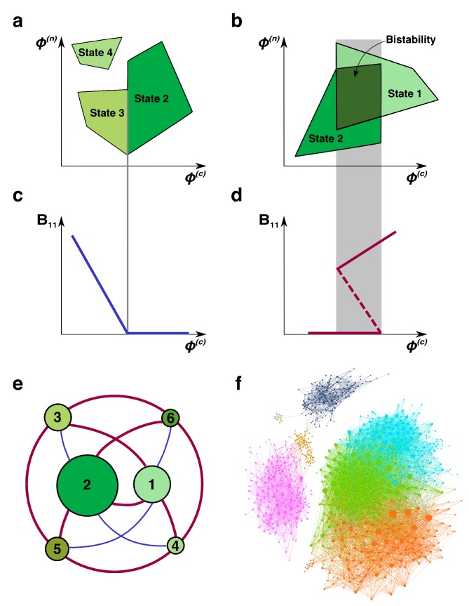
Figure 2. Regime shifts between alternative stable states.

(a) Shaded green areas schematically depict the feasible ranges of nutrient supply rates for several stable states in our model (#2-#4 in Figure 1B). The feasible range of the state #4 does not overlap with that of any other state. Feasible ranges of states #2 and #3 also do not overlap but share a common boundary. Panel (b) depicts the opposite scenario of overlapping feasible ranges of another pair of stable states (#1 and #2 in Figure 1B). In the overlapping region (dark green), they form a pair of alternative stable states. (c) A smooth transition between two states at the boundary. The population $B_{11}$ of the microbial species (1,1) is plotted as a function of changing nutrient supply rate ${\varphi }^{(c)}$ (same as the x-axis in panel (a)). Vertical gray line corresponds to the boundary between states #3 and #2. (d) A regime shift between two states. $B_{11}$ is plotted as a function of nutrient supply ${\varphi }^{(c)}$ as it sweeps through the overlapping region (gray area) in panel (b). Note abrupt changes of $B_{11}$ at the boundaries of the overlapping region and its hysteretic behavior as expected for regime shifts. Dashed line corresponds to $B_{11}$ in a dynamically unstable state (#7 in Figure 1B). (e) The network of possible regime shifts between pairs of stable states in the 2C × 2N × 4S model. Each red edge represents a possible regime shift between two states it connects (overlap of their feasible ranges as in panel (d)). Each blue edge corresponds to a smooth transition between two states while changing the fluxes (as in panel (c)). Nodes correspond to six uninvadable and dynamically stable states (state labels are the same as in Figure 1b). Sizes of nodes reflect relative magnitudes of feasible ranges of states they represent. (f) Network of 8633 possible regime shifts between pairs of 893 uninvadable dynamically stable states in the 6C × 6N × 36S model. The size of each node reflects its degree (i.e. the total number of other stable states that a given state can shift into). The color of each node corresponds to its network modularity class calculated as described in Materials and methods.

Figure 2—figure supplement 1. Statistics of pairwise bistability network for 6C × 6N × 36S example.

(a) Degree distribution of the network in Figure 2F. (b) Rank-ordered distribution of weights of network edges from Figure 2F. The weights of the network in Figure 2F are given by normalized overlaps between states.