Figure - PMC

Skip to main content

An official website of the United States government

Here's how you know

Here's how you know

Official websites use .gov
A .gov website belongs to an official government organization in the United States.

Secure .gov websites use HTTPS
A lock ( ) or https:// means you've safely connected to the .gov website. Share sensitive information only on official, secure websites.

View full-text article in PMC

. 2019 Nov 22;10:5292. doi: 10.1038/s41467-019-13228-9

Search in PMC
Search in PubMed
View in NLM Catalog
Add to search

© The Author(s) 2019

Open Access This article is licensed under a Creative Commons Attribution 4.0 International License, which permits use, sharing, adaptation, distribution and reproduction in any medium or format, as long as you give appropriate credit to the original author(s) and the source, provide a link to the Creative Commons license, and indicate if changes were made. The images or other third party material in this article are included in the article’s Creative Commons license, unless indicated otherwise in a credit line to the material. If material is not included in the article’s Creative Commons license and your intended use is not permitted by statutory regulation or exceeds the permitted use, you will need to obtain permission directly from the copyright holder. To view a copy of this license, visit http://creativecommons.org/licenses/by/4.0/.

PMC Copyright notice

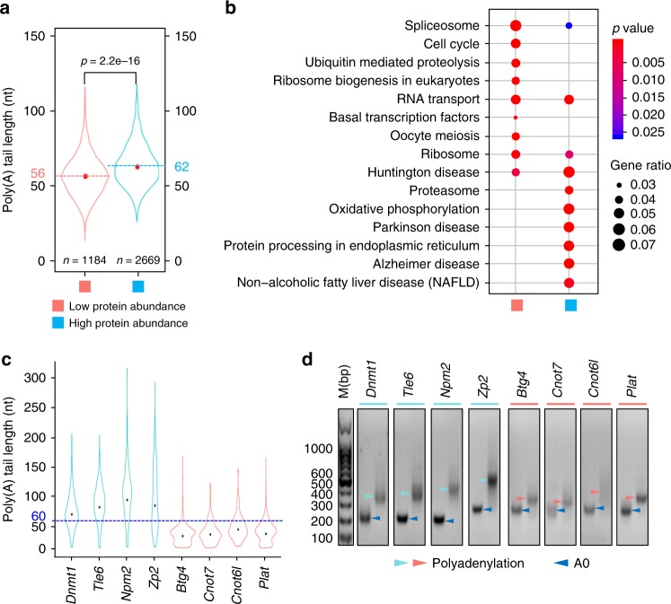
Fig. 4 — The length of poly(A) tail positively correlates with protein level. a Violin plot for poly(A) tail length distribution of low protein abundance and high protein abundance genes (genes with at least ten detected transcripts are included in the analysis). The two dotted lines represent the mean lengths of poly(A) tails of low protein abundance genes (pink) and high protein abundance genes (light blue). The p value was calculated by unpaired and two-sided Student’s t test. b Functional categorization of genes in high protein abundance gene and low protein abundance gene clusters by the KEGG pathway analysis (p value cutoff = 0.05). The p value is calculated by hypergeometric test. c Poly(A) tail length distributions for four high protein abundance genes (Dnmt1, Tle6, Npm2, and Zp2, cyan) and four low protein abundance genes (Btg4, Cnot7, Cnot6l, and Plat, pink). A blue dotted line indicating 60 nt used to help visualization of the poly(A) tail length difference between high protein abundance and low protein abundance gene groups. The black points indicate the mean poly(A) tail length of each gene. The number of CCS reads used are 390 (Dnmt1), 287 (Tle6), 146 (Npm2), 144 (Zp2), 685 (Btg4), 94 (Cnot7), 73 (cnot6l), and 413 (Plat). d Validation of the poly(A) tail length of the genes shown in Fig. 3c by PAT assay. The dark blue arrowheads represent bands with no poly(A) tail (A0), and the cyan (high protein abundance) and the pink (low protein abundance) arrowheads represent bands with poly(A) tail (polyadenylation). M, marker. Due to additional G tailing and adaptor sequence, the length of polyadenylation PCR products minus A0 products is at least 35 bp longer than the actual poly(A) tails⁴³. Source data are provided as a Source Data file.