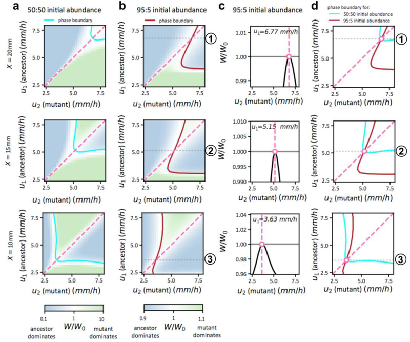
Extended Data Figure 8: Fitness landscapes for the competitive expansion process at different positions.

The position-dependent fitness landscapes for the competition between two strains (strain 1 and 2, e.g., an ancestor and a mutant), with expansion speeds u₁ and u₂ respectively, computed according to the competitive expansion model described in Extended Data Fig. 6a. The fitness of the mutant (strain 2) relative to the ancestor (strain 1) is defined as the ratio of its density with respect to the ancestor, i.e., $W(X)\equiv {\lim }_{t\to \infty }\left[\frac{{\rho }_2(X,t)}{{\rho }_1(X,t)}\right]$. In practice, we take t= 24 ℎ, which is well after the dynamics have halted. We further normalize this fitness by the ratio of the initial inoculant, $W_0\equiv \frac{{\rho }_2(X,0)}{{\rho }_1(X,0)}$, to obtain the “relative fitness gain”, W/W₀, which is plotted in various plots above. As indicated by the color bar at the bottom of the figure, green indicates a gain in the fitness of the mutant (W/W₀ > 1), while blue indicates loss of mutant fitness (W/W₀ < 1). The top, middle, and bottom rows refer to results at distances X = 20 mm, 15 mm,10 mm, respectively. a, The plots in the first column show the landscape W/W₀ for equal abundance (50:50) of the two strains at equal inoculation, i.e., W₀ = 1. The cyan and dashed lines are the two special lines, W/W₀ = 1 and u₁ = u₂, respectively. For W₀ = 1, the cyan line is the crossover distance, i.e., X = d_×(u, u′) (corresponding to W = 1) as explained in Fig. 4. The middle row (X = 15mm) is a zoomed out view of Fig. 4c, with a difference that the phase diagram in Fig. 4c only shows qualitative information on which strain dominates, whereas the fitness landscape here also provides quantitative information on the fitness gain. The top and bottom panel shows the corresponding fitness landscapes for X = 20 mm and X = 10 mm. b, The fitness landscape calculations are repeated for a mutant:ancestor inoculant ratio of 5:95 (i.e., W₀ ≡ ρ₂(X, 0): ρ₁(X, 0) = 5: 95). The solid brown line still indicates the phase boundary W/W₀ = 1, but it is no longer directly related to the crossover distance; see below. We see that the topological features of the landscapes in columns 1 and 2 are similar, but the details are different, reflecting the frequency-dependent nature of this competition process. c, In the 3^rd column, we plot the landscape profiles for 3 special ancestor expansion speeds, one at each position X, as indicated by the dotted grey lines marked by circled ① ② ③ in panel b, each obtained as the intersection of the phase boundary and the diagonal (solid brown line and the dashed pink line, respectively). Let us focus on the middle row (X = 15mm): For ancestral speed $u_1^{\ast }=5.15\hspace{0.17em}\hspace{0.17em}mm/h$ marked by grey line ②, the fitness landscape has a maximum at $u_2=u_1^{\ast }$ as marked by the white circle. This indicates that the ancestral expansion speed $u_1^{\ast }$ is stable to invasion by mutants with smaller or larger expansion speeds. Similarly, for X = 20 mm (top row), the ancestral speed $u_1^{\ast }=6.77\hspace{0.17em}\hspace{0.17em}mm/h$ marked by ① is the stable expansion speed, whereas for X = 10 mm (bottom row), the ancestral speed $u_1^{\ast }=3.63\hspace{0.17em}\hspace{0.17em}mm/h$ marked by ③ is the stable expansion speed. d, The phase boundaries shown as the solid cyan and brown lines in panels a,b turn out to intersect the diagonal at the same speed u^∗ for each X. Thus, the stable expansion speeds can be obtained from the crossover distance (cyan line) based on 50:50 inoculant, i.e., the relation (3) in the main text, despite the frequency dependence of the competition process. In other words, even though the overall fitness W depends on the initial frequency W₀ in a complex way, in the vicinity of the diagonal (u₁ ≈ u₂), W is independent of W₀ so that the simple illustration in Fig. 3a on the stability of a strain of speed u at distance d_×(u, u) is verified explicitly in panel c and d. To vary expansion speeds in each panel, the chemotactic coefficients c_i were varied within the range 180‥1500μm²/s. Diffusion coefficients were changed accordingly, D_i= c_i/6.25; see Supplementary Model and Supplementary Table 3.