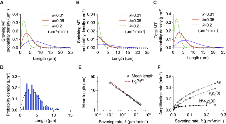
Figure 3.

Numerical solution of the steady-state severing model with dynamic instability. Distributions of growing (A) and shrinking (B) microtubules computed numerically from the ODEs (Eqs. 14 and 15) with boundary conditions (Eq. 22) are plotted for three different severing rates k. The dynamic parameters used for the solution are contained in Table 1. More frequent cutting leads to the shortening and compaction of length distribution. (C) The total microtubule length distribution, which is the sum of distributions in (A) and (B). The steady-state distributions from the stochastic simulations (k = 0.05 μm⁻¹⋅min⁻¹) are shown as open circles in (A)–(C) and agree with the ODE solutions. The proportion of shrinking microtubules is much smaller than that of growing microtubules, so the total distribution is similar to the growing one. (D) A comparison of the experimental length distribution (blue histogram (19)) with the predicted length distribution (dashed line, k = 0.05 μm⁻¹⋅min⁻¹). Both distributions have a mean length of ∼4 μm $\approx \sqrt{v_{\text{g}}/k}$. (E) Log-log plot of the mean length as a function of the severing rate. The open circles are the mean length obtained from the numerical solution. Black line is the linear regression of log k and $\log \overline{x}$ (R² > 0.9999). Red dashed line indicates (v/k)^1/2 of the no-catastrophe model case in which v = v_g = 0.79 μm/min. (F) Severing rate k vs. the amplification rate $k\overline{x}$ − v_sp_s(0⁺) (solid circles), the average number of cuts on a single microtubule $k\overline{x}$ (open circles), and the microtubule disappearance rate v_sp_s(0⁺) (squares). These three functions all increase with severing activity, but the amplification rate quickly reaches a plateau. To see this figure in color, go online.