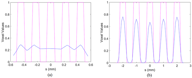
Figure 5.
Examples for determining the peak and valley regions for calculating the mean contrast values. The blue curve shows the profile of the reconstructed horizontal line pairs for Source 2. The magenta curve shows the ideal profile of the line pairs with the normalized peak voxel value of 1. The spatial frequencies are (a) f = 4.5/mm, (b) f = 1/mm. The slopes of the ideal profiles are not perfectly vertical because of the finite sampling rate of the profiles.

