Complex Acoustic Environments: Review, Framework, and Subjective Model

Abstract

The concept of complex acoustic environments has appeared in several unrelated research areas within acoustics in different variations. Based on a review of the usage and evolution of this concept in the literature, a relevant framework was developed, which includes nine broad characteristics that are thought to drive the complexity of acoustic scenes. The framework was then used to study the most relevant characteristics for stimuli of realistic, everyday, acoustic scenes: multiple sources, source diversity, reverberation, and the listener’s task. The effect of these characteristics on perceived scene complexity was then evaluated in an exploratory study that reproduced the same stimuli with a three-dimensional loudspeaker array inside an anechoic chamber. Sixty-five subjects listened to the scenes and for each one had to rate 29 attributes, including complexity, both with and without target speech in the scenes. The data were analyzed using three-way principal component analysis with a (2 3 2) Tucker3 model in the dimensions of scales (or ratings), scenes, and subjects, explaining 42% of variation in the data. “Comfort” and “variability” were the dominant scale components, which span the perceived complexity. Interaction effects were observed, including the additional task of attending to target speech that shifted the complexity rating closer to the comfort scale. Also, speech contained in the background scenes introduced a second subject component, which suggests that some subjects are more distracted than others by background speech when listening to target speech. The results are interpreted in light of the proposed framework.

Introduction

Recent hearing research has shown a growing interest in the effects that realistic listening conditions may have on different psychoacoustic measures, which are traditionally tested in the laboratory (Best, Keidser, Buchholz, & Freeston, 2015; Naylor, 2016; Neuhoff, 2004; Plomp, 2002). The realistic settings are often referred to as “complex acoustic environments” (CAEs), although different variations of this term are routinely encountered in the literature (see Table 1). While the central role that CAEs play in realistic hearing has been acknowledged in the current research, the exact meaning of the term and what it designates have remained opaque. This is addressed here by first providing a brief literature review on CAEs in hearing research, which is then developed and expanded into a framework that summarizes the key aspects that make an acoustic environment complex. This framework is then applied to stimuli that are used in an exploratory study to evaluate the perceived complexity of a range of realistic environments that are reproduced in the laboratory.

Table 1.

Different Wording Used in the Literature to Designate Complex Acoustic Environments.

Complex	Acoustic	Environment
Realistic	Auditory	Scenario
Everyday	Listening	Scene
Demanding	Multitalker	Soundscape
Challenging	Multisource	Condition
Adverse	Sound	Situation
Real world		Setting
		Field

CAEs in the Literature

The concept of CAEs did not fully make it to the mainstream jargon of hearing research until recent times, although it first appeared much earlier in different variations (Carhart & Tillman, 1970; Durrant, 1967; Harrison & Beecher, 1969; Tillman, Carhart, & Nicholls, 1973). The main boost to the eventual popularity of the term has likely been the seminal work by Bregman (1990) about auditory scene analysis. Even though he did not use the term explicitly in his book, a follow-up paper (Bregman, 1993) explained: “The simple rules for spatial perception that classical psychophysics has discovered by testing listeners in simple, quiet environments cannot be applied without modification in acoustically complex ones” (p. 16). Listeners have evolved to continuously segregate sound events from their environments, which they achieve either by using learned schemas unconsciously, attentively, and voluntarily or by following regularities in acoustic streams, such as common temporal and harmonic patterns—attributable to a single source. Similarly, Yost (1991) referred to “complex sound fields” as containing more than one source, from which the hearing system creates auditory images. A more in-depth review on the link between auditory scene analysis and CAEs that includes additional usages of the term in acoustics and related fields can be found in Weisser (2018).

Even though CAEs are often considered in the same vein as realistic acoustic environments, many of the hearing studies that picked up the CAE terminology did not necessarily attempt to construct realistic environments. Instead, they rather aimed at creating more involved scenes in terms of the scene analysis challenge using traditional psychoacoustic stimuli (e.g., Bendor & Wang, 2006; Pelofi, De Gardelle, Egré, & Pressnitzer, 2017; Wilson & Strouse, 2002; Zwiers, Van Opstal, & Cruysberg, 2001). However, there have been mounting concerns that observations collected using traditional psychoacoustic and audiometric methods, which may not exert subjects’ cognitive systems as realistically as complex environments do, have low predictive power to daily situations (e.g., Arlinger, Lunner, Lyxell, & Kathleen Pichora-Fuller, 2009). The cocktail party paradigm (Cherry, 1953), in which listeners are able to attend to a specific talker among several competing talkers in their immediate environment, is thus deemed a more appropriate model for realistic listening conditions. It is, however, a challenging problem to study in controlled conditions (McDermott, 2009; Middlebrooks, Simon, Popper, & Fay, 2017) and one that is not very well handled by current hearing aid technology (Shinn-Cunningham & Best, 2008). Cherry suggested a number of mechanisms that enable listeners to segregate the multiple talkers. Segregating multiple talkers has been a recurrent theme in auditory scene analysis research, sometimes emphasizing reverberation or variable source to background levels as factors that specifically add complexity to the scenes (e.g., Faller & Merimaa, 2004; Girolami, 1998; Hawley, Litovsky, & Colburn, 1999; Kamkar-Parsi & Bouchard, 2011; Lesser, Nawab, & Klassner, 1995; Ma, Milner, & Smith, 2006).

The higher level attention-related tasks of auditory scene analysis and object formation were gradually merged with the everyday cocktail party problem (Best, Ozmeral, Kopčo, & Shinn-Cunningham, 2008). It has been repeatedly reported that listening to speech in CAEs is a prime interest of hearing-device users, but a situation that is difficult to assess using common experimental techniques (Ghent, 2005; Naylor, 2016). This notion was explored in different studies using highly elaborate acoustic setups to be able to deal with multiple simultaneous sources distributed in space, reverberation, audio-visual displays, as well as elaborate signal processing. These studies obtained results that were at odds with traditional tests performed in simpler environments (e.g., Best et al., 2015; Brungart, Cohen, Cord, Zion, & Kalluri, 2014; Brungart, Sheffield, & Kubli, 2014; Smeds, Wolters, & Rung, 2015).

Few attempts have been made to narrow down the scope that is entailed by the CAE concept. With hearing aid evaluation difficulties as the focus, Ghent (2005) proposed a straightforward definition for complex sound fields: “sound fields created with at least two uncorrelated sound sources on different axes that result in sound wave interference at the center of the listening position. A simple sound field, by contrast, has a single sound source.” According to Ghent, the CAEs are confined to enclosed spaces with an isotropic and homogenous propagation medium, of constant acoustic impedance. Different classes of environments are drawn according to the kind of acoustic fields: free, diffuse, anechoic, reverberant, and real sound fields, which are dynamic, uncontrollable, and unpredictable. These real sound field properties are largely missing from measurements obtained in the laboratory, which is one possible reason they often fail to predict real-life performance of hearing aids. A speech-communication-centric take on the problem was offered by Mattys, Davis, Bradlow, and Scott (2012), who were concerned with types of “adverse conditions.” In their formulations, adverse conditions occur at the source, receiver, and environment. The environment-related degradation may be the result of noise sources that mask the speech or distraction caused by informational masking. These problems may be further exacerbated due to reverberation or noisy electronic transmission channels, whenever amplification is used. In all cases, stream segregation becomes more difficult and may overload the listener’s working and short-term memory.

While the discussion about complex environments in the acoustic literature has been formulated independently of the complexity literature, complex systems are widespread in the real world and some of their most well-known features are relevant to CAEs as well (Mitchell, 2009). Complexity science has been grappling with the existence of a universal definition of complexity across scientific domains (Lloyd, 2001; Mitchell, 2009, Chapter 7). Therefore, complex systems are often described using a particular subset of characteristics out of many that are commonly associated with complexity (Badii & Politi, 1999, Chapters 1–2). One such important feature of complex systems that has not been explicitly mentioned earlier is the different levels of connection and interaction between the various elements of a complex system that define its overall information dynamics, as is characteristic for networks (Strogatz, 2001). Applied to acoustic environments, an example of such a network would be a group of people talking, whereby they interact with one another through conversation. Their overall acoustics and conversation dynamics does not resemble that of the same people talking to themselves in one space—a dialog is not the aggregate of two monologs (Branigan, Catchpole, & Pickering, 2011; Schober & Clark, 1989). Moreover, the talkers will adapt their behavior to the acoustic environment that may contain background noise or other people talking, which provides an additional level of interaction that is commonly described by the Lombard effect (Lombard, 1911). In the case of other interfering talkers, the Lombard effect will influence the behavior of all talkers, who may iteratively raise their voices to make themselves understood until an equilibrium is reached or they (temporarily) give up talking.

CAE Framework

Based on the literature summarized earlier, an attempt is made in the following to frame what makes an acoustic environment complex. The resulting CAE framework can be employed as a tool that enables a comprehensive qualitative characterization of arbitrary acoustic scenes in terms of their acoustic complexity, as will be illustrated further. The framework was conceived to be as exhaustive and inclusive as possible so that the complexity of arbitrary acoustic environments can be accounted for using its characteristics.

With reference to Mattys et al. (2012), an acoustic environment is defined as bounded region in space that contains at least one sound source and one receiver, coupled through an acoustic medium (typically air; Ghent, 2005). Using this generic definition, it is suggested that the complexity of an acoustic environment can be exhaustively accounted for according to the nine broad characteristics listed in Table 2 or a subset thereof. The first three characteristics (multiple sources, source diversity, and source–source interaction) are related directly to the acoustic sources, with emphasis on delineating complex sources and complex environments. Characteristics 4 and 5 (reverberation and nonuniform medium) relate to the environment itself—the boundary conditions and the acoustic medium within which sound propagates in the system. Characteristics 6 to 8 (sound systems, source–environment adaptation, and other cues) present additional interactions that may exist between sources and environments. The last characteristic (receiver’s task) relates specifically to the receiver but informs and contextualizes the other characteristics. Overall, realism or everydayness is not necessary attributes that make a situation complex. It is possible to synthetically produce scenes with multiple sounds that are not normally heard outside of the laboratory, nor is a situation required to be challenging to be considered complex. For example, a conversation between three people in a quiet room may be considered a somewhat complex scene but is trivial for a normal-hearing listener to follow.

Table 2.

The Complex Acoustic Environment Framework.

Type	No.	Characteristic	Description
Source	1	Multiple acoustic sources distributed in space	The more acoustic sources that are present, the more independent streams of sound event information are competing for the listener’s attention (e.g., Cherry, 1953; Hawley et al., 1999; Shinn-Cunningham & Best, 2008).
	2	Acoustic source diversity	Sounds vary in temporal and spectral characteristics, radiation patterns, and position. The more variable the source is the more challenging it may be for the receiver to process these changes in the real time (e.g., Ghent, 2005; Sueur, Farina, Gasc, Pieretti, & Pavoine, 2014).
	3	Source–source interaction	Human talkers and other biological sound sources form interactive communication networks, so the sound produced by several sources (e.g., talkers) is not the same as each of them alone (McGregor, 2005).
Environment	4	Reverberation, reflections, scattering, diffraction, and diffusion	The geometry and materials of the environment, and objects within it, impose the boundary conditions on the propagation of sound that deviate from free-field acoustics. This blurs individual sound sources (e.g., Houtgast & Steeneken, 1985) and may make sound signals more difficult to hear in noise or competing signals (e.g., Brungart, Sheffield, et al., 2014; see Characteristic 9 later).
	5	Nonuniform medium for sound propagation	The medium can be inhomogeneous, nonlinear, nonisotropic, absorptive, and dispersive. This is mostly applicable for underwater acoustics, although over very long distances, large temperature gradients, precipitation, or turbulent conditions, some of these phenomena can become relevant to airborne sound as well (Daigle, 1979; Lengagne & Slater, 2002; Morton, 1975; Wiener & Keast, 1959).
Source–environment interactions	6	Loudspeaker amplification systems	Electronic amplification interacts with the room acoustics and affects the sound pressure levels and radiation patterns of sounds in space (Kuttruff, 2009, Chapter 10).
	7	Source–environment adaptation	Biological sound sources may react and adapt to the general acoustical conditions in the environment including reverberation, and general noise level, as well as their distribution in space (e.g., the Lombard effect, Lombard, 1911).
	8	Cues of other modalities	Sensory signals of different modalities tend to co-occur in natural settings and they can be combined and integrated by the receiver (Partan & Marler, 1999), and inform action (Lewicki, Olshausen, Surlykke, & Moss, 2014).
Receiver	9	Receiver’s task	The instantaneous task of the listener frames how much complexity matters (Badii & Politi, 1999, p. 6; Gell-Mann, 1995, p. 33), and how important the other characteristics (1–8) are within that context, given the receiver’s resources and knowledge.

The characteristics of the CAE framework sometimes require knowledge about the sources and the context that goes beyond their acoustics. Most notably, the source–environment–receiver delineation is not always applicable in practice. From the standpoint of the receiver, the environments and the sources can be inseparable. Also, the roles of sources and receivers are dynamic, as in a dialog, for instance, either of the interlocutors can be the listener and talker at times. Finally, the complexity of the medium in which they occur may be emulated using headphones that provide equivalent auditory cues. This can dissociate the spatial perception from the physical space outside the listener and thereby creates an environment completely localized around (or even inside) the listener’s head. The very last characteristic—the receiver’s task—is critical to framing all other characteristics, as it provides a context to the action of interest that takes place in the CAE system. This has recently been highlighted in a review by Lewicki et al. (2014) who noted that information gathered in ecologically valid (and biologically relevant) scene analysis must be directed by a particular goal of the perceiver. This, in turn, leads to modification of the perceiver’s actions in accordance with the information received through its senses and previous knowledge in memory.

Goals

The overarching goal of this study is to understand the factors that are most relevant for the subjective perception of complexity in acoustic scenes. This would allow a more effective use of CAEs in hearing research and thereby provide hearing outcomes with increased ecological validity. To achieve this goal, first, the CAE framework proposed earlier was applied to assess the characteristics of complexity that are most salient in everyday environments, considering a sample of 14 realistic acoustic scenes. These acoustic scenes were then used within an exploratory subjective experiment, which was designed with the specific aim to understand what listeners make out of the notion of complexity and how they deal with various aspects thereof. Subjects were asked to perceptually analyze the different acoustic scenes and to rate their perceived complexity as well as 28 additional subjective attributes. The responses were analyzed using a three-way principal component analysis (PCA) to reveal the most dominant connections between the acoustic scenes, rated attributes, and subjects.

Experimental Methods

Test Subjects

Sixty-five subjects participated in the test (48 females and 17 males) with an age range between 19 and 64 years (median 23 years). Subjects either had their hearing screened in the last year or were screened before the test began. Fifty subjects had normal hearing (pure tone thresholds below 20 dB HL at standard frequencies between 250 and 8000 Hz), and 15 had slight-to-mild losses (pure tone average, thresholds measured across 500, 1000, 2000, and 4000 Hz between 20 and 30 dB HL). Subjects were compensated for their participation either by payment or by course credit, if they were undergraduate students.

Test Setup

All stimuli were presented to the subjects using the 41-channel loudspeaker array located inside the anechoic chamber of the Australian Hearing Hub, Macquarie University, Australia. This spherical loudspeaker array is constructed from rings of equally spaced Tannoy V8 loudspeakers (Tannoy, Coatbridge, Scotland) at different elevation angles and a distance of 1.87 m from the center of the array (see Oreinos & Buchholz, 2016). All signals were processed on a PC at a sampling frequency of 44.1 kHz using MATLAB software and were presented to the subjects via an RME MADI PCIe sound card connected to two RME 32-channel M-32 digital-to-analog converters (RME, Haimhausen, Germany), which drove the 41 loudspeakers via 11 Yamaha XM4180 power amplifiers (Yamaha, Hamamatsu, Shizuoka, Japan). The power spectrum and sensitivity of each Tannoy loudspeaker were individually equalized using 2,048-sample long minimum-phase finite-impulse response filters. An additional Genelec 8020C loudspeaker (Genelec, Iisalmi, Finland), which was driven by the same audio system, was placed in front of the listener at a distance of 0.66 m to reproduce the direct sound of nearby target speech. This was required only for Part C of the questionnaire described later. The differences in sensitivity and distance of the nearby Genelec 8020C and the array loudspeakers were adjusted by applying a compensation gain and delay.

Realistic Acoustic Environments

To understand the factors that determine the perceived complexity of acoustic environments, 12 2-min samples of real-world urban scenes were taken from the Ambisonic Recordings of Typical Environments (ARTE) database (Weisser et al., 2019). The scenes represent a sample of typical urban environments that are encountered, more or less regularly, by many city dwellers (in this case, inhabitants of Sydney, Australia). Therefore, the sample was considered to cover a broad range of perceived complexity in everyday listening. All scenes naturally contained different amounts and types of acoustic sources from different directions were situated either indoor or in combined indoor–outdoor environments and exhibited a broad range of average sound pressure levels (SPLs). In addition to these real-world scenes, two speech-weighted Diffuse-Noise scenes were included to represent the type of masking noise that is common in psychoacoustic research and to serve as control conditions. The root-mean-square level of the Diffuse-Noise scenes was arbitrarily set to 58.3 and 68.3 dB SPL. An overview of the scenes is provided in Table 3, and a detailed description of the applied recording and processing methods is provided in Weisser et al. (2019).

Table 3.

The Complex Scene Stimuli Used in the Experiment, Which Were Taken From the ARTE Database.

	Scene name	Description	SPL (dB)	SPL (dBA)	T30 (s)	Speech (dBA)
1	Library	University study area in the main library, off-peak hours, quiet, distinctly audible acoustic objects, people whisper to avoid disturbing others.	53.0	46.1	0.6	54.6
2	Office	Open space office, people typing, chatting and talking on the phone	56.7	51.4	0.2	63.9
3	Diffuse Noise 1	Low-level speech-weighted broadband diffuse sound field L	58.3	54.2	N/A	62.7
4	Church 1	Small church space, people entering and chatting quietly before service	60.5	54.7	1.2	62.4
5	Living Room	Living room with access to kitchen in the back, loud television and sounds from the kitchen	63.3	58.7	0.2	65.0
6	Church 2	Same as 4, but busier and louder conversations (1.5 min)	65.9	60.9	1.2	67.5
7	Diffuse Noise 2	Medium-level speech-weighted broadband diffuse sound field	70	65.9	N/A	69.7
8	Café 1	Indoor café at medium occupancy	71.0	67.3	1.1	72.1
9	Café 2	Indoor (company) café at medium occupancy before lunch, next to the wall	71.7	66.2	1.1	70.8
10	Dinner Party	Small room with eight people chatting over the table with background music	72.8	68.7	0.4	71.8
11	Street/Balcony	Apartment balcony over a busy arterial road; Mainly traffic noise with some noise from within the apartment	74.5	71.1	N/A	75.6
12	Train Station	Sydney Central, main concourse—large space, open to the platforms with people walking at peak hour; loud amplified announcement and train sounds	77.1	73.6	1.0	74.2
13	Food Court 1	Busy university food court	78.2	74.9	0.9	74.9
14	Food Court 2	Very noisy food court in a shopping mall during lunch	79.6	76.7	1.0	76.6

Note. The scene names and descriptions are provided along with the unweighted (dB SPL) and A-weighted (dBA) SPLs, and the reverberation time T₃₀. Data in the table are reproduced from Weisser et al. (2019). The right-most column contains the target speech levels from 0.66 m in dBA. SPL = sound pressure level; N/A = not applicable.

To further understand the characteristics of the acoustic scenes with respect to their complexity, the scenes were classified using the CAE framework described earlier. This classification was performed qualitatively by the first two authors and involved their background knowledge from when the original scenes were recorded, acoustic measures from the original environments (e.g., RT₆₀), and subjects’ responses from Part A of the questionnaire described later. The results are described later and are summarized in Table 4.

Table 4.

A Qualitative Breakdown of Relevant CAE Framework Characteristics for the ARTE Scenes Described in Table 3.

	Scene name	CAE framework characteristic
		Multiple sources	Source diversity	Source–source interaction	Reverberation	Nonuniform medium	Amplification	Adaptation	Other modalities	Receiver’s task
		1	2	3	4	5	6	7	8	9
1	Library	+	+	+	−	−	−	+	−	+
2	Office	+	+	+	−	−	−	+	−	+
3/7	Diffuse Noise 1 and 2	−	−	−	−	−	−	−	−	+
4	Church 1	+	−	+	+	−	−	+	−	+
5	Living Room	+	+	−	−	−	+	−	−	+
6	Church 2	+	−	+	+	−	−	+	−	+
8/9	Café 1 and 2	+	+	+	+	−	+	+	−	+
10	Dinner Party	+	+	+	+	−	+	+	−	+
11	Street/Balcony	+	+	−	−	0	−	−	−	+
12	Train Station	+	+	+	+	0	+	+	−	+
13 /14	Food Court 1 and 2	+	+	+	+	−	−	+	−	+

Note. This breakdown gathers the most salient dimensions according to which perceived complexity may vary. The CAE framework characteristics are shown in Table 2. A plus (+) indicates that the respective characteristic was judged to be highly relevant to the scene, whereas a minus (−) indicates the opposite. The zero (0) indicates that a nonuniform medium effect (5) may have been present but could not be captured with the recording technology used. CAE = complex acoustic environment.

Realistic Speech Material

According to the proposed CAE framework described earlier (Table 2, Characteristic 9), the subject’s task may have a significant effect on the perceived complexity of an acoustic scene. Therefore, the effect of attending to speech while rating the complexity of the different scenes was evaluated in addition to a general scene analysis task. To implement this task, a modified set of the 14 acoustic scenes described earlier was generated, which also contained natural speech that could have been experienced in the original scenes in the real world.

Realistic target speech material

The target speech was extracted from recordings from Weisser and Buchholz (2019), which were obtained by applying the methods for eliciting natural conversations between two people described in Beechey, Buchholz, and Keidser (2018). In brief, subjects were asked to follow a puzzle task that could only be solved by communicating information between each other. While performing this task, the subjects were listening to binaural versions of the aforementioned acoustic scenes, one at a time, which were presented to them at their original SPL (Table 3) via highly open Sennheiser HD 800 headphones (Sennheiser, Hanover, Germany). As is expected from the Lombard effect, the conversation partners adjusted their vocal effort level (and other acoustic, linguistic, and communicative characteristics of their speech) to the individual acoustic scenes. During this conversation task, the subjects were seated on chairs in an anechoic chamber at a mouth-to-ear distance of approximately 1 m, facing each other, and their voices were recorded using calibrated DPA d:fine FIO66 omnidirectional headset microphones (DPA Microphones, Allerød, Denmark). The recorded conversations were later mapped to a recording distance of 1 m, by applying a negative gain, using the method described in Beechey et al. (2018). Moreover, 2-min recordings from one representative female talker, whose speech levels were close to the mean of 12 female talkers and had a pleasant voice, were then edited to obtain natural low-contextual single-talker conversational speech with scene-specific vocal effort level. The final edits were typically 35-45 s long and were therefore repeated to match the durations of the 2-min long scenes.

Realistic sound source properties of the target speech

The target speech edits were set to a realistic SPL and presented from a realistic distance along with matching reverberation. This follows observations by Pearsons, Bennett, and Fidell (1977, Figure 22), which suggest that talkers stand closer to one another the higher the background noise level is with an increase in effective speech level as a result. The realistic talker distances and target speech levels were derived from Weisser and Buchholz (2019), where conversational speech levels were recorded at 0.5 m and 1 m talker distance for the same 12 acoustic environments applied here. Thereby, it was assumed that the realistic talker distance is 1 m for the softest environment (the Library) and 0.5 m for the loudest environments (Food Court 2), which is slightly different from the distances of 0.9 m and 0.4 m derived in Weisser and Buchholz. For all other acoustic environments of intermediate noise levels, the target speech levels and talker distances were derived using a linear interpolation on a double-logarithmic scale (the abscissa being the SPL in dB and the ordinate the log distance). The resulting target speech levels are summarized in Table 3.

Realistic reverberation

For each of the 12 acoustic real-world scenes (excluding the Diffuse Noise scenes), the derived target speech material was convolved with a corresponding 41-channel room impulse response (RIR) from the ARTE database (Weisser et al., 2019). The RIR was measured in the same acoustic environment as the recorded scene using a Tannoy V8 loudspeaker at an azimuth angle of $0\circ$ at a distance of 1.3 m from the microphone array. Before convolution with the target speech, the direct sound component of each of the RIRs was separated from the reverberant component by applying a frequency-dependent time window (Weisser et al., 2019). The direct sound component was then summed across all 41 loudspeaker channels and assigned to an additional loudspeaker (Genelec 8020C) that was placed inside the loudspeaker array in front of the listener at a distance of 0.66 m—a distance that corresponded to that of a scene with a median SPL of the target talker across all scenes. The reason for this extra loudspeaker is that the robust reproduction of nearby sound sources, that is, sound sources that are significantly closer to the subject than the playback loudspeakers (here 1.87 m), is difficult to realize using loudspeaker arrays (Favrot & Buchholz, 2012). Moreover, presenting the target speech from a separate, clearly visible, nearby loudspeaker made it easier for the test subjects to focus on the corresponding speech within the acoustic scene. The direct and reverberant portions of the target speech were amplified differentially to account for the fact that the direct and reverberant fields are reproduced from different loudspeakers, but assuming that the direct field follows the inverse square law, whereas the reverberant field is independent of the source–receiver distance. The complete signal was amplified to produce the target speech levels shown in Table 3. Then, only the reverberant part was attenuated to account for the different distance between the measured RIR at 1.3 m and the assumed target speech at 0.66 m, applying a gain to the reverberation of $20\text{log}(0.66\text{m}/1.30\text{m})=-5.9$ dB. More detailed information on the involved methods can be found in Weisser and Buchholz (2019).

Questionnaire

While listening to the acoustic scenes, the subjects were asked to fill out a questionnaire, which was divided into three parts that together covered from different angles all relevant aspects of complexity as were identified in the CAE framework. Part A served primarily as a scene familiarization round. It required the listeners to analyze the scenes by asking them to identify as many sounds as they could, classified into categories (e.g., human-made, kitchen, traffic) and subcategories (e.g., footsteps, dishes, moving cars). Subjects were also asked to guess what the scene is. Only summary data from this part were used here and details are described in Weisser (2018, Chapter 4). Once the subjects felt familiar enough with the scene, they proceeded to Part B, where the scene identity and location were revealed to the subjects. This part contained 19 rating questions, relating to various subjective attributes of the scenes, such as familiarity, loudness, busyness, annoyance, reverberance, pleasantness, or how hard it would be to follow a conversation on the phone. An explicit rating of perceived complexity was obtained as one of the final questions without any further explanation. The subjects were also not informed that the complexity rating was of any higher importance in comparison with other ratings. Part C was similar to B, but with a nearby target talker added to the scene just in front of the subject. While listening to the target speech, subjects answered 10 additional rating questions, such as self-estimated speech intelligibility, listening effort, and complexity of the scene given the specific (additional) task of listening to the target speech.

The questionnaire that was used in this study was the result of multiple reiterations by the authors based on pilot field and laboratory trials. Special attention was paid to refrain from using jargon in the question wording so that they could be easily understood by lay subjects. The full questionnaire is provided in Online Appendix A.

Procedure

Test subjects were seated at the center of a loudspeaker array in an anechoic chamber, while listening to three-dimensional recordings of real acoustic scenes. The recordings were 2 min long but played in a loop for as long as the subjects needed to complete the tasks. While listening to the scenes, subjects filled in (paper) questionnaires—one per scene—that probed into different attributes of the scenes. The playback system was optimized to the listener’s head position, but subjects were free to turn their heads to better focus on sounds when needed. A single training scene (Café 2 in Table 3) opened the test to familiarize the subjects with the questionnaire and concept of the test. Then, seven scenes were presented in a random order, followed by a mandatory break. In the second half of the test, seven more scenes were presented in a random order, the first of which was a repetition of one of the first seven scenes. As the data measured for the training scene were found to be as stable as for all other scenes, data for a total of 14 scenes (plus one repeated condition) were evaluated in this study. Each scene was repeated twice every 13 subjects. The entire test took 1.5 to 3 h per subject.

Statistical Modeling

Data Preparation

The raw data that were obtained from the questionnaire, as well as its preparation for statistical analysis, are described later. The unprocessed data array contained 31,850 observations out of which 178 points (0.56%) were missing. The data provided 36 observed variables, including 30 rating scales (1 question from Part A, 19 questions from Part B, and 10 questions from Part C), the test time for Part A and Part B combined, the test time for Part C, the scene presentation order, and three scales derived from Questions #1 to #3, that is, the nominal count of sound events, the nominal count of talking people (i.e., the estimated number of individual talkers in the scene), and a combined recognition score. In the following, all 36 variables will be collectively referred to as “scales.”

As these 36 scales measured fundamentally different quantities, they were not directly comparable and therefore only their relative variability was taken into account in the data analysis. Scales that were not in the standard rating range of 0 to 10 were therefore equalized to fit that range (Kroonenberg, 2008). Moreover, data that were not directly derived from a rating scale had to be transformed into an effective (equalized) rating score. Answers to the distraction questions specifically (#12 and #25) may have not been directly comparable because they often referred to different sounding objects. Nevertheless, to enable comparison, this aspect was ignored and where no distraction was reported, the rating was set to zero.

The nominal count of sound events scale was derived from the responses to Question #1 (excluding #1 a) by calculating the sum of all distinct events (or categories, in cases where subjects did not go into subcategorical details) that were identified by the subjects in each scene. Similarly, the nominal count of talking people was calculated from the identified number of people talking (Question #1 a). The latter count was constrained by the maximum number of people talking that the question allowed, whereby the “more than three people” option was counted as four events. These two scales were summed up to yield a combined nominal count of sound events that will be referred to as “event count” from here on. This reduced the total number of scales to 35.

It is unclear how many sound events (including talking people) that subjects recognized could be mapped to actual events in reality and whether their identification was correct (Weisser, 2018, Chapter 5). To take this aspect into account, a combined recognition score was derived from the subjects’ responses to Questions #1 to #3. As the “ground truth” about the number and type of events that were present in the original (real) scenes is unknown, a proxy measure was applied based on a “white list” that was iteratively developed by four experienced listeners. Based on a complete list of all the events that were identified by the subjects for all the scenes, these listeners eliminated all those events that they could not hear when carefully and repeatedly listening to the scenes. The resultant list was then screened again by a different group of four experienced listeners. The remaining events then formed the “white list.” Using this list and the knowledge of what the scene was, a combined recognition “event score” was calculated based on successfully identified attributes of the scene: 1/2 point was given for each correctly identified event category, 1 point for each event (or event sub-category), 2 points for the environment type, and 4 points for the scene location. While this score is somewhat arbitrary, it provided a simple way to include the binary recognition data as an additional variable. For example, a subject who was presented with the office scene and correctly identified more than three people talking, laughter and ventilation noise, and correctly classified that it was recorded indoors in an office received 12 points in total: 6 points for events, 2 points for environment type, and 4 points for location. It should be noted that because two Diffuse Noise and Church scene variations were presented, the place and space type recognition scores were counted only in their first presentations, as in many cases learning improved the scene identification performance in their second presentation.

All rating data were centered to zero and normalized to unity variance according to procedures explained in Kroonenberg (2008, Chapters 6 and 14) and Weisser (2018).

Tucker3 Model Selection and Simplification

The subjective data that resulted from the questionnaire were analyzed using a Tucker3 three-way PCA model (Tucker, 1966). Tucker3 modeling enables the reduction of high-dimensionality data to lower dimensionality, which is easier to interpret than the unreduced data, and can be associated with actual aspects of the stimuli and experiment. In the present analysis, this allowed the exploration of the variances of the three types of data involved in the results, as well as their interactions, that is, the 35 scales (rating question, object counts, test duration, and other variables), 14 scenes (acoustic environments or conditions), and 65 subjects. Each one of these types is referred to as a “mode” and represents a fundamentally different aspect of the data, which is not directly comparable with the other types (Kroonenberg, 2008, p. 28; Smilde, Bro, & Geladi, 2005, pp. 2–4). Simpler methods than three-way PCA would have required averaging data over modes and thereby removed information that could be important (Jolliffe, 2002, pp. 397–399; Thompson, 2004, p. 84). The Tucker3 method was selected over alternative three-way methods because it is particularly suitable for modeling rating data (Kroonenberg, 2008, Chapter 14; Murakami & Kroonenberg, 2003). The Tucker3 analysis method is described in more detail in Online Appendix B. All data modeling and analyses were performed using the N-Way toolbox for MATLAB (Andersson & Bro, 2000).

The Tucker3 analysis produced principal components, which can be thought of as the quintessential variables of each mode. To identify the three-way model that involves the lowest number of principal components while still accounting for the main behavior of the data, the scree plot of Figure 1 should be considered. This plot describes the variability accounted for in Tucker3 models using different combinations of components. The triplets on the plot refer to the number of modal components (scale scene subject). By definition, any PCA always lists the largest component first, which corresponds to a (1 1 1) model. The most informative point on the plot is where the addition of new components does not add any significant information anymore by modeling with more principal components. This appears in Figure 1 either at (2 3 2) or (2 3 3), where a knee point shows as the curve turns and asymptotically approaches 100% of explained variability. The (2 3 2) model turned out to be much more parsimonious than the (2 3 3) model and allowed a coherent interpretation within the theoretical and empirical framework of the experiment, as it contained only three elements in the core array—the three-dimensional array that weighs and combines the different modes to produce data points (see Online Appendix B). Henceforth, only the (2 3 2) model will be discussed. The final model—two of the three component loading matrices—and the simplified core array (Tables 5, 7 and 8) constitute the complete model parameters.¹ These parts of the model will be described in “Results” section. The explicit Tucker3 model ${\stackrel{\sim }{x}}_{\mathit{ijk}}$ is described as follows:

$$\begin{array}{c}{\stackrel{\sim }{x}}_{\mathit{ijk}}=a_{i1}{g}_{111}{c}_{j1}{b}_{k1}+a_{i2}{g}_{221}{c}_{j1}{b}_{k2}+a_{i1}{g}_{132}{c}_{j2}{b}_{k3}\end{array}$$ (1)

where the elements a, b, c, and g relate to the loading scale matrix A, scene matrix B, subject matrix C, and the core array G, respectively. The indices i, j, and k run through all scale $1\le l\le 35$, scene $1\le l\le 14$, and subject $1\le l\le 65$ data points, respectively. The first term on the left connects the first scale, scene, and subject components; the second term connects the second scale and scene with the first subject components, whereas the last term connects the first scale with the third scene and second subject components. See “Results” section for a detailed analysis.

Figure 1.

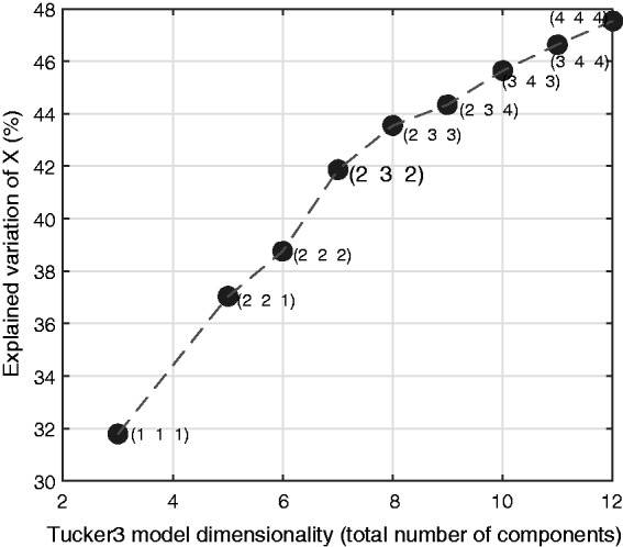
Scree plot of different component combinations of Tucker3 models. The triplets on the plot designate the number of components for scales scenes subjects. The amount of explained variation is measured as percentage of the sum of square differences between the original data set to the fitted one. The final model that was selected (2 3 2) is emphasized.

Table 5.

The Core Array, G, of the (2 3 2) Tucker3 Model, Simplified by Forcing the Smallest Terms to Zero.

	Scene 1	Scene 2	Scene 3
Subject Component 1
Scale 1	99.65	0.00	0.00
Scale 2	0.00	41.30	0.00
Subject Component 2
Scale 1	0.00	0.00	−38.87
Scale 2	0.00	0.00	0.00

Table 7.

The Loading Matrix A of the Two Scale Components, Grouped According to the Clusters They Form on the Joint Biplot in Figure 2.

	Scale Component 1	Scale Component 2
Pleasantness	0.141	−0.088
Intelligibility	0.177	−0.126
Loudness	−0.176	0.137
Phone listening	−0.229	0.107
Annoyance	−0.212	0.198
Annoyance speech	−0.242	0.046
Attention	−0.211	0.027
Stress	−0.185	0.074
Disturbance speech	−0.255	0.068
Focus	−0.193	0.045
Focusing speech	−0.224	0.033
Fatigue	−0.218	0.148
Fatigue speech	−0.250	0.066
Effort speech	−0.254	0.041
Difficulty speech	−0.200	0.096
Difficulty	−0.070	0.051
Variability	−0.133	−0.386
Familiarity	−0.097	−0.416
Realism	−0.059	−0.299
Event count	−0.051	−0.321
Event score	−0.010	−0.249
Realism speech	−0.070	−0.263
Complexity	−0.199	−0.176
Complexity speech	−0.234	−0.150
Effort	−0.173	−0.073
Busyness	−0.217	−0.129
Distraction	−0.175	−0.099
Distraction speech	−0.242	−0.098
Distinction	0.072	−0.245
Presentation order	0.002	0.129
Time AB	−0.011	−0.090
Time C	−0.016	−0.045
Envelopment	−0.036	0.092
Spaciousness	−0.035	0.108
Reverberance	−0.077	0.054

Table 8.

Loading Matrix of the Three Scene Components (B).

	Scene Component 1	Scene Component 2	Scene Component 3
Library	0.413	−0.353	0.117
Office	0.135	−0.207	0.377
Diffuse Noise 1	0.411	0.456	0.147
Church 1	0.224	0.000	0.231
Living Room	0.119	−0.257	0.298
Church 2	0.086	0.123	0.426
Diffuse Noise 2	0.223	0.559	0.261
Cafe 1	−0.118	−0.255	0.296
Cafe 2	−0.083	−0.261	0.199
Dinner Party	−0.057	−0.006	0.341
Street/Balcony	−0.318	0.155	0.221
Train Station	−0.210	−0.100	0.286
Food Court 1	−0.407	0.112	0.186
Food Court 2	−0.432	0.226	0.150

Note. The first component mainly drives the comfort ratings, whereas the second drives the variability. The third component is only required to reveal the second subject component (see later).

Results

Acoustic Scene Classification

The CAE framework was applied to the 14 ARTE scenes to break down their complexity into the nine characteristics described in Table 2. The results are summarized in Table 4. This breakdown is coarse-grained, as it imposes a binary classification of characteristics that can vary continuously. This was done on purpose to indicate whether these aspects appear significant in the scenes or not and thereby to guide and inform the design of the exploratory study described later, including the analysis of the resulting data.

The information on multiple sound sources (1) and sound source diversity (2) was taken from an analysis of the data from Part A of the questionnaire (see later), where the subjects were asked to identify all the sound sources they could hear in the individual scenes. As shown in Table 4, all recorded scenes contained multiple sources, and most of them provided significant source diversity. The number of identified sources that were confirmed by expert listeners (see earlier), and also used as a scale in the main experiment (see later), ranged from two sources (i.e., many people talking and sibilant speech) in Church 2 (#6) to 18 sources in Café 1 (#9; Weisser, 2018, Chapter 5). The most dominant sources are mentioned in Table 3. Source–source interaction (3) was present in most scenes and mainly referred to conversations between two or more people. Reverberation (4) was also present in most scenes, and, if applicable, the corresponding reverberation time (RT₆₀) is given in Table 3, ranging from 0.2 s in the Living Room (#5) to 1.2 s in the Church (#4 and #6). Nonuniform medium for sound propagation (5) was not addressed. Even though strong winds in some of the original recordings of the semiopen environments (i.e., the Train Station #11 and the Street/Balcony #12) may have resulted in a nonuniform medium, the wind also corrupted the microphone array recordings (Weisser et al., 2019) and the corresponding sound samples could not be utilized here. Loudspeaker amplification systems (6) were present in some scenes, and mostly referred to incidental music or television, except for the Train Station (#12), where an amplified announcement dominated a part of the scene. All observed source–environment adaptation (7) referred to the Lombard effect, except for the library, where people whispered due to social norms. Cues of other modalities (8) were not addressed because the study only considered audio recordings. The receiver’s task (9) was part of the design of the main experiment and is addressed in the next subsection.

As evident from Table 4, the acoustic scenes varied along seven different complexity characteristics, although the combination of possible characteristics did not vary systematically between scenes. Moreover, the diffuse noise scenes were devoid of any obvious complexity according to the CAE framework and were mainly included as controls.

Model Prediction

The chosen (2 3 2) Tucker3 model explained 41.66% of the variability of the complete set of 31,672 data points collected from 65 subjects in 14 acoustic scenes using 35 scales from the developed complexity questionnaire. The robustness of model variability to outliers and missing data was cross-validated using a jackknife procedure (Jolliffe, 2002, pp. 120–127; Kroonenberg, 2008, pp. 188–189) and found only a 0.06% drop in explained variability when 1/9th or 1/13th of the data were replaced at random. Similarly, replacing the data in the array with the repeated condition for every subject (1/14th of the data) caused a maximum drop of only 1% in the explained variability. The repeated condition was used also to obtain a test–retest reliability measure using Pearson’s correlation between all replicated rounds over all variables and environments and their first presentation. The resulting correlation of R = .79 indicates a reasonable test–retest reliability (Crocker & Algina, 2008, pp. 131–146). Hence, the chosen (2 3 2) Tucker3 model was confirmed as a robust model of the data.

Core array

The core array of the (2 3 2) Tucker3 model was optimized for simplicity by forcing the minimally contributing elements to zero (see Equation 1)—costing only a 0.2% loss of explained variability (originally, 41.87%) through additional core array elements. The resultant three nonzero elements ($g_{111},g_{221},\text{\hspace{1em}and\hspace{1em}}{g}_{132}$) are given in Table 5 and represent the most salient connections between the two scale modes, three scene modes, and two subject modes of the (2 3 2) Tucker3 model. Table 6 gives the explained variation (sum of squares) that is distributed between the component connections. The core element g₁₃₂, for instance, refers to the Scale 1 component connected to the Scene 3 and Subject 2 component and explains 11.48% of the modeled data.

Table 6.

The Relative Contribution of the Core Array Elements to the Total Variation Explained by the Simplified (2 3 2) Tucker3 Model.

Core element gijk	Explained variation (%)	Value	Sum of squares
$g_{111}$	75.53	99.65	9,930
$g_{221}$	12.97	41.30	1,706
$g_{132}$	11.48	−38.87	1,510

Scale mode

The scale mode of the model has two principal components, which span the scale space and are plotted as vectors in the joint biplot of Figure 2, along with the first two scene components that are given as points (see later). Several clusters are visible, which are summarized in Table 7. Most ratings are organized along the angled x-axis in what could be considered a measure of perceived “Comfort,” as it maps on the left-side positive attributes: pleasant sounding (Question #22) and highly intelligible (with target speech, #26). On the right side, it maps most other attributes, which are generally uncomfortable: loud (#8), annoying (with and without target speech, #10, #27), fatiguing (with and without target speech, #17, #30), difficult with target speech (#28), difficult to listen to the phone (#9), stressful (#20), hard to focus (with and without target speech, #18, #29), disturbing during target speech (#24), difficult to maintain attention (#19), and effortful during target speech (#31). The second scale component lined up with the ratings of “variability” (#11) and is surrounded to its left by realism (with and without target speech, #6, #33), familiarity (#5), event count (#1), and event score (#1–#3). An additional cluster appears to contain combinations of the comfort and variability components: complexity (with and without target speech, #21, #32), busyness (#7), distraction (with and without target speech, #12, #25), and effort (without target speech, #23). The rating of “distinction” (#13) is also a combination of comfort and variability, but mirrored to the other side of the variability axis than complexity, which sets it apart. Finally, some attributes are obviously much weaker than others (shorter vectors represent smaller correlations) and do not map well to the two principal scale components. These are envelopment (#14), spaciousness (#15), presentation order, and test time to completion of Parts A + B and C. Both difficulty (to complete Part A, #4) and reverberance (#16) have similar direction as loudness and fatigue but are much weaker and therefore less dominant.

Figure 2.

Joint biplot of the scale and scene first and second components. The vectors represent the different scales, where names ending with (S) refer to target speech attributes in Part C of the questionnaire. The first two scene components are superimposed on the plot, with the large markers designating the scenes. If a marker is closer to a particular scale, then it is more closely related to that attribute. The biplot origin designates the average value of every scale over all scenes and subjects.

Scene mode

The loading matrix of the scene mode has three components (see Table 8). The first two components become clear when plotted together with the two scale components on a joint biplot (Figure 2) that illustrates how the two modes interact. The third scene component mainly helps to understand the differences between subjects and is further described later. The two scale and two scene components are connected through a single-subject component that is reflected in the two largest core array elements (see Table 5). The corresponding joint biplot was constructed by considering only part of the Tucker3 model, which contains a single “slice” r of the core array that connects the scene and scale matrices via ${\mathbf{AG}}_{\mathbf{r}}\mathbf{B}={\mathbf{A}}_{\mathbf{r}}^{*}{\mathbf{B}}_{\mathbf{r}}^{*}$. By then removing the second subject component, the core array G was reduced to the top 2 × 3 matrix G₁ of Table 5. Finally, G₁ was decomposed using the singular value decomposition of ${\mathbf{G}}_{\mathbf{r}}={\mathbf{U}}_{\mathbf{r}}{\mathbf{L}}_{\mathbf{r}}{\mathbf{V}}_{\mathbf{r}}\text{'}$ and its factors were divided between A and B (Kroonenberg, 2008, pp. 273–274) resulting in the following equation:

$${\mathbf{A}}_{\mathbf{r}}^{*}=(\frac{I}{J}{)}^{1/4}{\mathbf{AU}}_{\mathbf{r}}{\mathbf{L}}_{\mathbf{r}}^{1/2}{\mathbf{B}}_{\mathbf{r}}^{*}=(\frac{J}{I}{)}^{1/4}{\mathbf{BV}}_{\mathbf{r}}{\mathbf{L}}_{\mathbf{r}}^{1/2}$$ (2)

where the new components ${\mathbf{A}}_{\mathbf{r}}^{*}$ and ${\mathbf{B}}_{\mathbf{r}}^{*}$ are scaled according to the number of scales and scenes in the data to not bias their apparent length in the plot as they are unequal (i.e., I = 35 scales vs. J = 14 scenes). This operation effectively rotates and scales the components so that they can be projected onto a single plane and plotted together with the two scene components into a joint biplot (Figure 2). In this joint biplot, the distance between the scenes (points) and the scales (vectors), that is, the projection from the point to a vector, corresponds to how closely that scale describes the particular scene. As the weights of the core array also scale this projection, the joint biplot correctly displays the importance of the different components in relation to one another. Figure 2 therefore illustrates how the scene components can be understood through the overlaying scales. Similarly to the scale components, the first scene component accounts for scene pleasantness/comfort/noisiness and the second for scene richness/variability/familiarity in the second component.

Subject mode

Two subject components were considered to model the main features of the prototypical subject behavior. The first component is the most dominant one and, combined with the two scale and two first scene components in the core array, accounts for about 88.5% of the total core variability (sums of squares), which gives the average listener’s response. The second subject component accounts for the remainder of 11.5% (see Table 6) and represents a subset of the subjects that reacted differentially to some of the scenes. The second component is expressed only through the third scene component (Table 5), which suggests again that their combination is necessary to represent different subjective preferences about the scene attributes.

To get a handle on the meaning of the second subject component, it was examined how it correlates with different mean scale ratings throughout the test. Strong correlations (with $R^2>.5$) were found with phone listening (Question #9, $R^2=.51$), annoyance (#10, $R^2=.52$), fatigue (#17, $R^2=.54$), focus (#18, $R^2=.51$), stress (#20, $R^2=.54$), disturbance during speech (#24, $R^2=.66$), distraction during speech (#25, $R^2=.57$), annoyance during speech (#27, $R^2=.67$), focusing during speech (#29, $R^2=.72$), fatigue during speech (#30, $R^2=.73$), complexity during speech (#32, $R^2=.63$), and effort during speech (#31, $R^2=.78$), which is plotted in Figure 3. Therefore, the difference in behavior between subjects was evident mainly when they had to attend to speech or perform a speech-related task. However, not all scenes elicited this difference between subjects. If only the four scenes are analyzed that did not contain any obvious speech (the Library, two Diffuse Noise scenes, and Street/Balcony), all of the aforementioned R² values dropped below.2 to .3. In contrast, if only the scenes that were dominated by speech were analyzed (the Office, Church 1 and 2, Living Room, Café 1 and 2, Dinner Party, Train Station, and Food Courts 1 and 2), then the R² values stayed close to their original values. In summary, a small yet consistent difference was observed in how subjects reacted to background speech, as some subjects found it more difficult than others to accommodate to it. This is best seen in their higher self-reported listening effort when attending to target speech, which suggests that some people are more distracted than others by speech interferers and therefore may be also more susceptible to informational masking (Kidd, Mason, Richards, Gallun, & Durlach, 2008). No obvious predictors could be identified for why these subjects differ using demographic information available, such as age, hearing loss, and gender. It should be emphasized that the core array elements that are associated with this subject effect connect it to both the comfort and the variability scale components (in addition to the third scene component). Comfort is weighted 3 times more strongly than variability but both increase/decrease with background speech.

Figure 3.

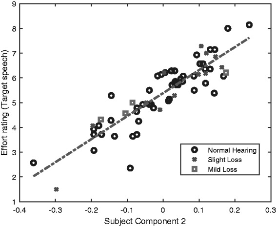
The strongest correlation of any rating scale to the second subject component was with the listening effort rating during speech. Only the scenes with dominant background speech drove this differentiation. Hearing status does not appear to consistently predict the mean subjective ratings (four subjects with mild losses, >25 dB HL, were grouped separately from the slight losses for illustration purposes only).

Additional Analyses

Complexity ratings

The main goal of this exploratory study was to identify the attributes that contribute to the perceived complexity of an acoustic scene. Thereby, it was inherently implied that subjects were able to consistently and meaningfully rate acoustic scene complexity without any further clarification or training. This was confirmed by the strong weighting of the complexity scale within the Tucker3 model (Table 7) as well as by the decent test–retest reliability, which found a Pearson’s correlation coefficient of R = .81 and R = .78 for the complexity with and without target speech, respectively (Questions #21 and #32). The quality of the complexity data is further illustrated by considering the spread of the mean complexity ratings shown in Figure 4 as a function of acoustic environment (with and without target speech) as well as the relatively small 95% confidence intervals shown by the error bars. The complexity data reveal that the subjects utilized almost the entire rating scale, and the nonoverlapping confidence intervals found between many environments indicate significant differences between those environments. It is interesting to note that in two scenes the complexity rating increased significantly when subjects were asked to attend to additional target speech, that is, the Living Room and the Street/Balcony scenes. Both had strong modulated maskers—television speech, or noisy traffic—that readily interfered with speech reception but were apparently less complex on their own. As Figure 2 reveals, the mean rating of busyness (#7) is very close in length and direction to the mean rating of complexity (#21). If the scene average is considered, then busyness and complexity have a correlation of $R^2=.97$ (no-target speech) and $R^2=.92$ (with target speech), whereas if the individual data are considered, then it drops to $R^2=.52$ and $R^2=.49$, respectively. Therefore, it appears that subjects closely associate the notions of scene busyness and complexity.

Figure 4.

The scene complexity ratings averaged over all 65 subjects, ordered by increasing sound pressure level (dB SPL) from left to right. The error bars are the Tukey–Kramer 95% confidence intervals of pairwise comparisons of all ratings.

General Discussion

Principal Component Analysis

Most of the observed data could be modeled using two principal components of the scale mode and their equivalent scene mode components as well as one subject component (i.e., five components in total). A persistent second subject component with its corresponding third scene component accounted for a smaller fraction of the total variation but highlighted an interesting subject effect.

The first and most dominant scale component, comfort, included on the negative end various unpleasant attributes that listeners rated highly in the environments—annoyance, disturbance, distraction, loudness, fatigue, stress, difficulty to focus, difficulty to attend to speech, or talk on the phone—and two positively phrased qualities on the other end—pleasantness and high speech intelligibility. These relations are in line with a previous survey that found subjective comfort to be associated closely with quiet–noisy and pleasant–unpleasant subjective ratings of outdoor urban soundscapes (Kang & Zhang, 2010). The loudness rating question (#8) referred explicitly to the sound being comfortable or uncomfortable (see Online Appendix A), although subjective comfort is not exactly equivalent to perceived noise level, despite a strong correlation (Yang & Kang, 2005). Nonequivalence between these two factors is also visible in Figure 2, which shows that loudness does not fully account for the comfort component, as they are not exactly collinear. Nevertheless, the comfort component is strongly driven by the acoustic energy in the scene, which in most cases was the result of many incoherent sources of the same type being mixed together. The food courts clearly contained many more people talking than the Church scenes, which contained more distinct and sporadic conversations. Similarly, the Street/Balcony scene had heavy traffic that contained numerous vehicles. The Library, in contrast, contained many different sound events, which were all relatively quiet.

The second scale component, variability, appears to be more suitable to describe the diversity of the sound events, rather than their quantity. The subjective ratings of variability itself, the nominal subjective event count, and the event score all fit this notion well. The Diffuse-Noise sound scenes, with their monotonous sound, were perceived as completely unvarying to all subjects, whereas the Café and Train Station scenes sounded highly variable. The inclusion of the diffuse sound field scenes was central in revealing this component.

The additional scales that mapped to the variability component, realism and familiarity, may have been inadvertently confounded by the choice of scenes. The Diffuse-Noise scenes contained the lowest number of sound events, but were also unfamiliar to almost all participants, and were judged to be completely unrealistic. The Church scenes were rated higher on realism and they contained more events (mostly conversations), but they generally did not represent a convincing prototypical church, which resulted in significantly lower ratings than for most of the other scenes (Weisser et al., 2019). This was largely due to its uncharacteristically low reverberation time of 1.2 s, the everyday contents of the conversations it captured, and the lack of any ceremonial cues, such as an ongoing sermon or live music. Moreover, many test subjects verbally reported that they are not church-goers, so they were unfamiliar with this environment to begin with. All other scenes, in comparison, contained more distinctly recognizable sound events and were rated to be much more familiar and realistic.

Reverberation, envelopment, and spaciousness neither mapped clearly onto the two scale components, nor did they result in an additional independent component. In general, these ratings did not vary much between the scenes. A possible explanation to that was the usage of the ambisonic reproduction system. All scenes were spatialized in the same way, so subjects may have reacted to that uniformity. Reverberation in the recorded scenes did vary significantly (Table 3), but may have been confounded with the overall level, as louder scenes tended to be recorded in larger spaces (the Street/Balcony being the notable exception). This can be noticed in the joint biplot of Figure 2, where reverberance is parallel to comfort. Nevertheless, the effect of reverberation on the sound events may have been secondary to their overall level. This can account for the low correlation between reverberance and comfort, which is seen in the short length of its vector compared with the others in the joint biplot.

The first two scale components, comfort and variability, are mirrored in the two scene components, as prototypical scenes may be placed somewhere on the plane that is described by the level of comfort and degree of variability they induce. The description is correct for the average listener, who is represented by the first subject component. However, the individual reaction to dominant background speech in the scenes systematically modulates this average response for a subset of the listeners. Modeling this effect requires the third scene and second subject components. Unfortunately, the third scene component does not map directly to any attribute in the scenes, but can only be understood as a necessary feature to reorder the ratings for the different scenes, when the second subject component is moved away from its mean value. These extra components therefore should be included in the modeling when dealing with environments that contain background speech, if individual variation is to be accounted for. Finally, additional factors such as familiarity, realism, or envelopment may all be valid attributes of scenes as well but could not be disentangled from others with the scenes selected in this study.

The rating of subjective distinction of sound events in space is set apart—halfway between the components, but in opposite direction to complexity on the comfort axis—may also be interpreted in light of the above. Quieter scenes with fewer sound events, that is, rated of higher comfort, are usually indicative of sparser auditory displays, which enable easier stream segregation, a quality that was referred to as “hi-fi soundscapes” (Schafer, 1994, pp. 43–44). The contribution of the variability component to distinction may be that sound event diversity facilitates segregation. For example, segregating one out of many talkers is a more difficult task than distinguishing between a coffee machine and background music.

Perceived Scene Complexity

Subjects had no difficulty relating to the term scene complexity and reliably rating it, and they closely associated it with busyness. This can be seen by having complexity ratings that are both interpretable and reproducible. In addition, the test subjects did not ask for any clarifications regarding the questions related to complexity. Complexity turned out to be composed of at least two separate components. The ratings of the subjective complexity shifted when the task focus was switched from a more general scene analysis in Parts A and B of the questionnaire to the target speech in Part C. In the latter case, it was more strongly affected by the comfort component and was driven very close to the ratings of scene busyness and distraction. Possibly, this is because speech reception is more susceptible to masking by other speech (Kidd & Colburn, 2017; Kidd et al., 2008). Further examination of the subject components showed that the degree to which subjects were affected by speech in the relevant scenes was individual. However, the between-subject source of variation is unknown. It is possible that using a more fine-tuned selection of scenes, extra dimensions of complexity that are hidden now might appear, such as familiarity and envelopment. Also, scene complexity generally increased with loudness (Figure 4)—a natural side effect of having more acoustic sources in the environment. By artificially matching the levels of different scenes, another hidden aspect of the perceived complexity may be revealed. Only the Diffuse-Noise scenes were repeated at two levels, where the louder presentation (68.3 dB SPL) was rated as slightly more complex than at a lower presentation level (58.3 dB SPL). Level-dependent complexity rating difference was insignificant (half a rating point) for no-target speech, one-way analysis of variance $p>.05,F(1,128)=2.69$, and significant (one full point) with target speech, $p<.01,F(1,128)=13.91$.

Subjective Complexity and the CAE Framework

All in all, the CAE framework was successfully employed to qualitatively describe diverse acoustic situations and identify their potential sources of complexity in a systematic way that would have been difficult to attain otherwise. The analysis with the applied statistical model directly addressed at least four of the nine characteristics of the CAE framework (Table 2), although only three proved to contribute significantly to subjective complexity.

The comfort component of the derived statistical model is highly related to the first characteristic of the framework, “Multiple acoustic sources distributed in space,” at least in environments where high acoustic energy is associated with multiple sources, as was the case in most of the considered scenes. This was indeed the most dominant characteristic that was hypothesized to be relevant to the scenes (see Table 4). This is in line with findings by Ghozi, Fraj, Salem, and Jaidane (2015), where the number of similar sources was shown to partially drive the complexity estimates in a survey of university cafeteria during lunch. In that study, the respondents’ rated complexity was correlated with the approximate number of people present in the surveyed cafeteria during lunch, which would be considered a measure of comfort in this study. Interestingly, the objective complexity of that scene, which was estimated from audio recordings using an entropy measure, also correlated with the occupancy level in the cafeteria.

Similarly, the variability component of the derived statistical model may be understood as a direct measure of the second characteristic of the framework, “Acoustic source diversity.” In contrast, reverberation, a central component of the fourth characteristic of the CAE framework, could not be clearly resolved from other features of the scenes and needs to be further investigated using additional or different scenes.

The “receiver’s task” characteristic (9) directly affected the perceived complexity when the subjects shifted from general unfocused listening to the scenes (questionnaire Part B) to attending to the target speech (questionnaire Part C; see Figure 2). The receiver’s task had an additional variation in the form of the sound events distinction rating (Question #13), which may be seen as a fundamentally different task to the explicit complexity rating, as it required an analytic listening to sound objects, rather than synthetic listening to the entire scene. It is simpler to perform when the events sound very different from one another and the environment is quieter and also when the sound events are more familiar. The effect can be seen in Figure 2, where the direction of the distinction and complexity vectors are mirrored against the variability axis.

Many potential sources of complexity as encompassed by the other CAE framework characteristics were not addressed by the applied stimuli. Even though it is possible to generate stimuli that vary on these complexity dimensions, the role such intricate acoustics may have in making hearing-relevant situations sound more complex is unknown. This means that variants of perceived scene complexity exist that are not covered by these stimuli and are not addressed in this study. However, adding more systematic variations in complexity would have been in conflict with the main approach of this study, that is, to use a set of different realistic everyday scenes.

Limitations

At this point, it is still unknown how the subjective components derived from the statistical model relate to acoustic measures that are inherent to the scenes and their recordings. Whereas the comfort component is strongly related to the SPL of the environments, it is unclear how variability can be best measured acoustically. A successful measures may need to quantify the temporal, spectral, and spatial variability of the acoustic scenes as captured by the auditory system. Therefore, it is likely that hearing loss will have an effect on such a complexity measure, as it is typically accompanied by degraded temporal acuity, spectral selectivity, and spatial resolution. A more quantitative approach will be necessary if realistic scene complexity is to be integrated in more advanced hearing research and hearing-device design and evaluation, where a growing interest in real-world performance drives much of the present work. Future research will have to address this aspect in depth.

Several aspects of this work may limit its generalizablity. By design, this study excluded all visual cues from the virtual environment presentations. This, along with the somewhat unusual task that lacks robust context for the listener, arguably constrains the ecological validity of the test, and therefore the level of realism that can be achieved with this particular method. This concern may be exacerbated by the particular choice of questions that went into the questionnaire that may create an unknown bias in the subjective data obtained. That said, the subjects reported that the questionnaire was straightforward to use and many commented that they found the task engaging and stimulating because it related to situations that they are generally familiar with from everyday life. In addition, they found the sound reproduction generally very convincing. The lack of visual cues was noticed but at no point constituted an impasse to completing the task. Combined with the analysis that provided a sensible and interpretable model, it suggests that there is a great deal that may be learned about CAEs before adding other modalities. Finally, the scene selection may also constrain the generalization of the conclusions universally to arbitrary scenes—especially scenes recorded outdoors in nonurban settings. This aspect of the test also shows in the uneven treatment of different characteristics of the CAE framework. Selection may also limit the universality of the target speech used, which was one specific female voice, processed to sound realistic within the scenes. However, some subjects noted that the fact that the speech was shorter than the scene and repeated, made it sound less realistic.

Another possible limitation is the sound presentation method, which provides limited fidelity at high frequencies, in direct proportion to the order of the reproduction system. Ahrens, Marschall, and Dau (2018), for instance, showed that the order of a horizontal ambisonic system (lower and higher than the one used in this study) can influence the spatial resolution of sound sources, which may affect subjects’ apparent source width perception and speech intelligibility that follows spatial release from masking. It is possible that some of the busiest scenes presented in this study were therefore more spatially distorted than quieter scenes in a way that influenced a subset of the ratings. However, as was suggested earlier, the measured spatially related attributes contributed little to the variation and interpretation of the data as a whole.

Finally, modeling the scene-based subjective ratings required significant investment of time and attention from the listeners, which resulted in a large amount of data that are based on different individual references for ratings. Several factors that were not estimated, such as individual sensitivity to noise and spatial awareness, may have also contributed to the spread of data. This means that a substantial portion of the variation (58%) could not be efficiently modeled using the three-way PCA.

Conclusions

The present work systematically probed the complexity aspect in CAEs by proposing a general framework with nine characteristics (Table 2), along with an empirical method that tested the subjective evaluation of 14 realistic, everyday scenes. Three characteristics of the CAE framework dominated the variation in the acoustic scenes: multiplicity of sources (1), diversity of source types (2), and the listener’s task (9). The subjective results revealed two orthogonal components of scene complexity—comfort and variability—driven by the scenes themselves that were characterized as varying along the same two dimensions. An additional component was observed when the acoustic scenes included significant background speech that can distract the listener while attending to target speech. Some listeners reacted more strongly to this distraction than others, which affected some of their ratings in relevant scenes, particularly the listening effort rating while attending to target speech. Other characteristics such as the amount of reverberation (4) and interaction between the sources (3) may have not been dominant enough in the considered acoustic environments to generate a clear effect on the subjects’ ratings. Moreover, specific perceptual attributes such as realism, familiarity, and envelopment may have been confounded by the experimental design, and future studies will need to investigate whether their influence on perceived complexity is significant.

Overall, subjects reported that they related well to the task, despite the lack of visual cues and detailed explanations of the various attributes in the questionnaire. While being based on exploratory subjective ratings, these results were statistically reliable. It remains to be seen in a confirmatory study whether the long questionnaires can be reduced to a shorter one with less question redundancy, which may still enable the reliable quantification of the perceived scene complexity. It is suggested that the CAE framework and empirical methods can be utilized in hearing research and other relevant areas in acoustics to systematically explore additional aspects of complexity in real-world environments.

Declaration of Conflicting Interests

The authors declared no potential conflicts of interest with respect to the research, authorship, and/or publication of this article.

Ethical Approval

The behavioral measurements in this study complied with the ethics guidelines of the Australian Hearing Human Research Ethics Committee, approval number AHHREC2016-13.

Funding

The authors disclosed receipt of the following financial support for the research, authorship, and/or publication of this article: This study was funded by the Oticon Foundation and Macquarie University via an iMQRES PhD scholarship.

References

- Ahrens, A., Marschall, M., & Dau, T. (2018). The relation between source width perception and speech intelligibility with virtual sound sources. Paper presented at the 41st Annual Midwinter Meeting of the Association for Research in Otolaryngology, San Diego, CA.
- Andersson C. A., Bro R. (2000) The N-way toolbox for MATLAB. Chemometrics and Intelligent Laboratory Systems 52(1): 1–4. doi: 10.1016/S0169-7439(00)00071-X. [Google Scholar]
- Arlinger S., Lunner T., Lyxell B., Kathleen Pichora-Fuller M. (2009) The emergence of cognitive hearing science. Scandinavian Journal of Psychology 50(5): 371–384. doi: 10.1111/j.1467-9450.2009.00753.x. [DOI] [PubMed] [Google Scholar]
- Badii R., Politi A. (1999) Complexity: Hierarchical structures and scaling in physics (Vol, 6). Cambridge, England: Cambridge University Press. [Google Scholar]
- Beechey T., Buchholz J., Keidser G. (2018) Measuring communication difficulty through effortful speech production during conversation. Speech Communication 100: 18–29. doi: 10.1016/j.specom.2018.04.007. [Google Scholar]
- Bendor D., Wang X. (2006) Cortical representations of pitch in monkeys and humans. Current Opinion in Neurobiology 16(4): 391–399. doi: 10.1016/j.conb.2006.07.001. [DOI] [PMC free article] [PubMed] [Google Scholar]
- Best V., Keidser G., Buchholz J. M., Freeston K. (2015) An examination of speech reception thresholds measured in a simulated reverberant cafeteria environment. International Journal of Audiology 54(10): 682–690. doi: 10.3109/14992027.2015.1028656. [DOI] [PMC free article] [PubMed] [Google Scholar]
- Best V., Ozmeral E. J., Kopčo N., Shinn-Cunningham B. G. (2008) Object continuity enhances selective auditory attention. Proceedings of the National Academy of Sciences 105(35): 13174–13178, doi 10.1073/pnas.0803718105. [DOI] [PMC free article] [PubMed] [Google Scholar]
- Branigan H. P., Catchpole C. M., Pickering M. J. (2011) What makes dialogues easy to understand? Language and Cognitive Processes 26(10): 1667–1686. doi: 10.1080/01690965.2010.524765. [Google Scholar]
- Bregman A. S. (1990) Auditory scene analysis: The perceptual organization of sound, Cambridge, MA: MIT Press. [Google Scholar]
- Bregman A. S. (1993) Auditory scene analysis: Hearing in complex environments. In: McAdams S., Bigand E. (eds) Thinking in sound: The cognitive psychology of human audition, Oxford, England: Oxford University Press. doi: 10.1093/acprof:oso/9780198522577.001.0001, pp. 10–36. [Google Scholar]
- Brungart D. S., Cohen J., Cord M., Zion D., Kalluri S. (2014) Assessment of auditory spatial awareness in complex listening environments. The Journal of the Acoustical Society of America 136(4): 1808–1820. doi: 10.1121/1.4893932. [DOI] [PubMed] [Google Scholar]
- Brungart D. S., Sheffield B. M., Kubli L. R. (2014) Development of a test battery for evaluating speech perception in complex listening environments. The Journal of the Acoustical Society of America 136(2): 777–790. doi: 10.1121/1.4887440. [DOI] [PubMed] [Google Scholar]
- Carhart R., Tillman T. W. (1970) Interaction of competing speech signals with hearing losses. Archives of Otolaryngology 91(3): 273–279. doi: 10.1001/archotol.1970.00770040379010. [DOI] [PubMed] [Google Scholar]
- Cherry E. C. (1953) Some experiments on the recognition of speech, with one and with two ears. The Journal of the Acoustical Society of America 25(5): 975–979. doi: 10.1121/1.1907229. [Google Scholar]
- Crocker L., Algina J. (2008) Introduction to classical and modern test theory, Mason, OH: Cengage Learning. [Google Scholar]
- Daigle G. (1979) Effects of atmospheric turbulence on the interference of sound waves above a finite impedance boundary. The Journal of the Acoustical Society of America 65(1): 45–49. doi: 10.1121/1.382265. [Google Scholar]
- Durrant J. D. (1967) Effect of relevant cues on attention in binaural listening. The Journal of the Acoustical Society of America 41(6): 1613–1613. doi: 10.1121/1.2143735. [Google Scholar]
- Faller C., Merimaa J. (2004) Source localization in complex listening situations: Selection of binaural cues based on interaural coherence. The Journal of the Acoustical Society of America 116(5): 3075–3089. doi: 10.1121/1.1791872. [DOI] [PubMed] [Google Scholar]
- Favrot S., Buchholz J. M. (2012) Reproduction of nearby sound sources using higher-order ambisonics with practical loudspeaker arrays. Acta Acustica United With Acustica 98(1): 48–60. doi: 10.3813/AAA.918491. [Google Scholar]
- Gell-Mann M. (1995) The Quark and the Jaguar: Adventures in the simple and the complex, London, England: Macmillan. [Google Scholar]
- Ghent R. M. (2005) A tutorial on complex sound fields for audiometric testing. Journal of the American Academy of Audiology 16(1): 18–26. doi: 10.3766/jaaa.16.1.3. [DOI] [PubMed] [Google Scholar]
- Ghozi R., Fraj O., Salem M. B., Jaidane M. (2015) Occupancy-based analysis and interpretation of soundscape auditory complexity: Case of a campus restaurant. Journal of the Audio Engineering Society 63(6): 475–487. doi: 10.17743/jaes.2015.0057. [Google Scholar]
- Girolami M. (1998) A nonlinear model of the binaural cocktail party effect. Neurocomputing 22(1): 201–215. doi: 10.1016/S0925-2312(98)00058-7. [Google Scholar]
- Harrison J., Beecher M. (1969) Control of responding by the location of an auditory stimulus: Role of rise time of the stimulus. Journal of the Experimental Analysis of Behavior 12(2): 217–227. doi: 10.1901/jeab.1969.12-217. [DOI] [PMC free article] [PubMed] [Google Scholar]
- Hawley M. L., Litovsky R. Y., Colburn H. S. (1999) Speech intelligibility and localization in a multi-source environment. The Journal of the Acoustical Society of America 105(6): 3436–3448. doi: 10.1121/1.424670. [DOI] [PubMed] [Google Scholar]
- Houtgast T., Steeneken H. J. (1985) A review of the MTF concept in room acoustics and its use for estimating speech intelligibility in auditoria. The Journal of the Acoustical Society of America 77(3): 1069–1077. doi: 10.1121/1.392224. [Google Scholar]
- Jolliffe I. T. (2002) Principal component analysis (2nd ed.), New York, NY: Springer. doi: 10.1007/b98835. [Google Scholar]
- Kamkar-Parsi A. H., Bouchard M. (2011) Instantaneous binaural target PSD estimation for hearing aid noise reduction in complex acoustic environments. IEEE Transactions on Instrumentation and Measurement 60(4): 1141–1154. doi: 10.1109/TIM.2010.2084690. [Google Scholar]
- Kang J., Zhang M. (2010) Semantic differential analysis of the soundscape in urban open public spaces. Building and Environment 45(1): 150–157. doi: 10.1016/j.buildenv.2009.05.014. [Google Scholar]
- Kidd G., Jr., Colburn H. S. (2017) Informational masking in speech recognition. In: Middlebrooks J. C., Simon J. Z., Popper A. N., Fay R. R. (eds) The auditory system at the cocktail party, Cham, Switzerland: Springer International Publishing AG. doi: 10.1007/978-3-319-51662-2, pp. 75–109. [Google Scholar]
- Kidd G., Jr., Mason C. R., Richards V. M., Gallun F. J., Durlach N. I. (2008) Informational masking. In: Yost W. A., Fay R. R., Popper A. N. (eds) Auditory perception of sound sources, New York, NY: Springer. doi: 10.1007/978-0-387-71305-2, pp. 143–189. [Google Scholar]
- Kroonenberg P. M. (2008) Applied multiway data analysis, Hoboken, NJ: John Wiley & Sons. [Google Scholar]
- Kuttruff H. (2009) Room acoustics, 5th ed New York, NY: Taylor & Francis. [Google Scholar]
- Lengagne T., Slater P. J. (2002) The effects of rain on acoustic communication: Tawny owls have good reason for calling less in wet weather. Proceedings of the Royal Society of London B: Biological Sciences 269(1505): 2121–2125. doi: 10.1098/rspb.2002.2115. [DOI] [PMC free article] [PubMed] [Google Scholar]
- Lesser V. R., Nawab S. H., Klassner F. I. (1995) Ipus: An architecture for the integrated processing and understanding of signals. Artificial Intelligence 77(1): 129–171. doi: 10.1016/0004-3702(94)00033-W. [Google Scholar]
- Lewicki M. S., Olshausen B. A., Surlykke A., Moss C. F. (2014) Scene analysis in the natural environment. Frontiers in Psychology 5: 199. doi: 10.3389/fpsyg.2014.00199. [DOI] [PMC free article] [PubMed] [Google Scholar]
- Lloyd S. (2001) Measures of complexity: A nonexhaustive list. IEEE Control Systems Magazine 21(4): 7–8. doi: 10.1109/MCS.2001.939938. [Google Scholar]
- Lombard E. (1911) Le signe de l’elevation de la voix (The sign of the elevation of the voice). Annales Maladies Oreille, Larynx, Nez, Pharynx 37(101–119): 25. [Google Scholar]
- Ma L., Milner B., Smith D. (2006) Acoustic environment classification. ACM Transactions on Speech and Language Processing (TSLP) 3(2): 1–22. doi: 10.1145/1149290.1149292. [Google Scholar]
- Mattys S. L., Davis M. H., Bradlow A. R., Scott S. K. (2012) Speech recognition in adverse conditions: A review. Language and Cognitive Processes 27(7–8): 953–978. doi: 10.1080/01690965.2012.705006. [Google Scholar]
- McDermott J. H. (2009) The cocktail party problem. Current Biology 19(22): R1024–R1027. doi: 10.1016/j.cub.2009.09.005. [DOI] [PubMed] [Google Scholar]
- McGregor P. K. (2005) Animal communication networks, Cambridge, England: Cambridge University Press. doi: doi.org/10.1017/CBO9780511610363. [Google Scholar]
- Middlebrooks J. C., Simon J. Z., Popper A. N., Fay R. R. (2017) The auditory system at the cocktail party, Cham, Switzerland: Springer International Publishing AG. doi: 10.1007/978-3-319-51662-2. [Google Scholar]
- Mitchell M. (2009) Complexity: A guided tour, Oxford, England: Oxford University Press. [Google Scholar]
- Morton E. S. (1975) Ecological sources of selection on avian sounds. The American Naturalist 109(965): 17–34. doi: 10.1086/282971. [Google Scholar]
- Murakami T., Kroonenberg P. M. (2003) Three-mode models and individual differences in semantic differential data. Multivariate Behavioral Research 38(2): 247–283. doi: 10.1207/S15327906MBR3802_5. [Google Scholar]
- Naylor G. (2016) Theoretical issues of validity in the measurement of aided speech reception threshold in noise for comparing nonlinear hearing aid systems. Journal of the American Academy of Audiology 27(7): 504–514. doi: 10.3766/jaaa.15093. [DOI] [PubMed] [Google Scholar]
- Neuhoff J. G. (2004) Ecological psychoacoustics, San Diego, CA: Elsevier Academic Press. [Google Scholar]
- Oreinos C., Buchholz J. M. (2016) Evaluation of loudspeaker-based virtual sound environments for testing directional hearing aids. The Journal of the American Academy of Audiology 27(7): 541–556. doi: 10.3766/jaaa.15094. [DOI] [PubMed] [Google Scholar]
- Partan S., Marler P. (1999) Communication goes multimodal. Science 283(5406): 1272–1273. doi: 10.1126/science.283.5406.1272. [DOI] [PubMed] [Google Scholar]
- Pearsons, K. S., Bennett, R. L., & Fidell, S. (1977). Speech levels in various noise environments (Technical Report EPA600/1-77-025). Washington, DC: Office of Health and Ecological Effects, Office of Research and Development, U.S. Environmental Protection Agency.
- Pelofi C., De Gardelle V., Egré P., Pressnitzer D. (2017) Interindividual variability in auditory scene analysis revealed by confidence judgements. Philosophical Transactions of the Royal Society B: Biological Sciences 372(1714): 20160107. doi: 10.1098/rstb.2016.0107. [DOI] [PMC free article] [PubMed] [Google Scholar]
- Plomp R. (2002) The intelligent ear: On the nature of sound perception, Mahwah, NJ: Lawrence Erlbaum Associates. [Google Scholar]
- Schafer R. M. (1994) The soundscape: Our sonic environment and the tuning of the world, Rochester, VT: Destiny Books. [Google Scholar]
- Schober M. F., Clark H. H. (1989) Understanding by addressees and overhearers. Cognitive Psychology 21(2): 211–232. doi: 10.1016/0010-0285(89)90008-X. [Google Scholar]
- Shinn-Cunningham B. G., Best V. (2008) Selective attention in normal and impaired hearing. Trends in Amplification 12(4): 283–299. doi: 10.1177/1084713808325306. [DOI] [PMC free article] [PubMed] [Google Scholar]
- Smeds K., Wolters F., Rung M. (2015) Estimation of signal-to-noise ratios in realistic sound scenarios. Journal of the American Academy of Audiology 26(2): 183–196. doi: 10.3766/jaaa.26.2.7. [DOI] [PubMed] [Google Scholar]
- Smilde A., Bro R., Geladi P. (2005) Multi-way analysis: Applications in the chemical sciences, Hoboken, NJ: John Wiley & Sons. doi: doi.org/10.1002/0470012110.ch8. [Google Scholar]
- Strogatz S. H. (2001) Exploring complex networks. Nature 410(6825): 268–276. doi: 10.1038/35065725. [DOI] [PubMed] [Google Scholar]
- Sueur J., Farina A., Gasc A., Pieretti N., Pavoine S. (2014) Acoustic indices for biodiversity assessment and landscape investigation. Acta Acustica United With Acustica 100(4): 772–781. doi: 10.3813/AAA.918757. [Google Scholar]
- Thompson B. (2004) Exploratory and confirmatory factor analysis: Understanding concepts and applications, Washington, DC: American Psychological Association. [Google Scholar]
- Tillman T. W., Carhart R., Nicholls S. (1973) Release from multiple maskers in elderly persons. Journal of Speech, Language, and Hearing Research 16(1): 152–160. doi: 10.1044/jshr.1601.152. [DOI] [PubMed] [Google Scholar]
- Tucker L. R. (1966) Some mathematical notes on three-mode factor analysis. Psychometrika 31(3): 279–311. doi: 10.1007/BF02289464. [DOI] [PubMed] [Google Scholar]
- Weisser, A. (2018). Complex acoustic environments: Concepts, methods, and auditory perception (PhD thesis). Macquarie University, Sydney, Australia. doi: 1959.14/1266534.
- Weisser A., Buchholz J. (2019) Conversational speech levels and signal-to-noise ratios in realistic acoustic conditions. The Journal of Acoustical Society of America 145(1): 349–360. doi: 10.1121/1.5087567. [DOI] [PubMed] [Google Scholar]
- Weisser, A., Buchholz, J., Oreinos, C., Galloway, J., Beechey, T., Davila, J., & Keidser, G. (2019). The ambisonic recordings of typical environments (ARTE) database. Acta Acustica United With Acustica, 105(4), 695–713. doi: 10.3813/AAA.919349.
- Wiener F. M., Keast D. N. (1959) Experimental study of the propagation of sound over ground. The Journal of the Acoustical Society of America 31(6): 724–733. doi: 10.1121/1.1907778. [Google Scholar]
- Wilson R. H., Strouse A. (2002) Northwestern university auditory test no. 6 in multi-talker babble: A preliminary report. Journal of Rehabilitation Research and Development 39(1): 105. [PubMed] [Google Scholar]
- Yang W., Kang J. (2005) Acoustic comfort evaluation in urban open public spaces. Applied Acoustics 66(2): 211–229. doi: 10.1016/j.apacoust.2004.07.011. [Google Scholar]
- Yost W. A. (1991) Auditory image perception and analysis: The basis for hearing. Hearing Research 56(1): 8–18. doi: 10.1016/0378-5955(91)90148-3. [DOI] [PubMed] [Google Scholar]
- Zwiers M., Van Opstal A., Cruysberg J. (2001) A spatial hearing deficit in early-blind humans. The Journal of Neuroscience 21(9): RC142. doi: 10.1523/JNEUROSCI.21-09-j0002.2001. [DOI] [PMC free article] [PubMed] [Google Scholar]
Associated Data
This section collects any data citations, data availability statements, or supplementary materials included in this article.
Supplementary Materials
Supplemental material, TIA881346 Supplemental Material for Complex Acoustic Environments: Review, Framework, and Subjective Model by Adam Weisser, Jörg M. Buchholz and Gitte Keidser in Trends in Hearing