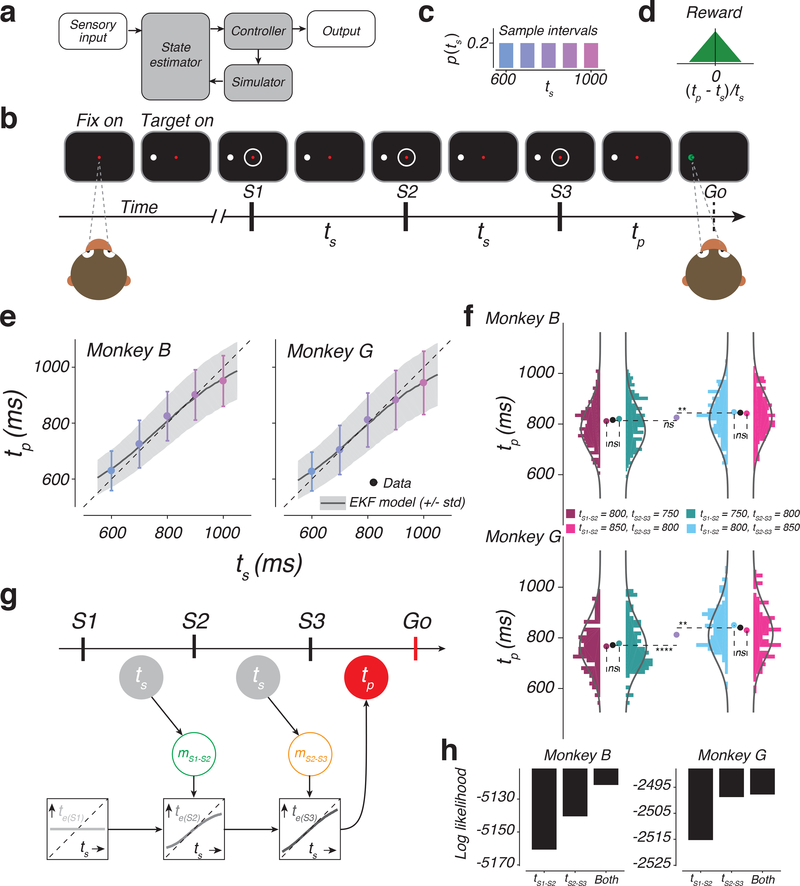
Figure 1. The 1-2-3-Go task, behavior, and a sequential updating model.

a) Internal-model based control. The controller drives the output. In the presence of delays and variability, the output control would benefit from a simulator and a state estimator. The simulator predicts the output and the estimator integrates the prediction with sensory inputs to update the controller. b) Sequence of events during a trial of 1-2-3-Go. The monkey fixates a central spot (Fix on). After the presentation of a saccadic target (Target on), three isochronous flashed annuli (S1, S2, and S3) are presented around the fixation point. The animal measures the sample interval (t_s), between consecutive flashes and aims to produce a matching interval (t_p) after S3 (Go). c) Sample interval distribution, p(t_s). Across trials, t_s was randomly drawn from a discrete uniform prior distribution with 5 values ranging between 600 and 1000 ms. d) Reward schedule. Maximum reward was delivered for t_p=t_s. Reward amount decreased linearly to zero with increasing relative error (|(t_p - t_s)/t_s|). e) Produced interval (t_p) as a function of sample interval (t_s). t_p increased monotonically with t_s (mean: colored circles; standard deviation: error bars; monkey B: n = 1412, 1326, 407, 1336, 1326 total trials for t_s = 600, 700, 800, 900, and 1000 ms, respectively; monkey G: n = 699, 724, 243, 685, 643 trials for t_s = 600, 700, 800, 900, 1000 ms, respectively). Responses were biased toward the median t_s and away from the unity line (dashed). Black traces and gray shadings are the mean and standard deviation predicted by the Extended Kalman Filter (EKF) model fit to the behavior. f) Analysis of behavior under the four cue conflict conditions. Histograms show the distribution of t_p in different cue conflict conditions (colors) for the two animals (top and bottom). Monkey B: n = 215, 216, 224, and 206 trials (left to right). Monkey G: n = 117, 83, 111, and 104 trials (left to right). Solid lines are the predicted distribution under the EKF model. Pairs of nearby histograms (e.g., t_S1-S2 = 800 ms, t_S2-S3 = 750 ms versus t_S1-S2 = 750 ms, t_S2-S3 = 800 ms) correspond to conflict conditions with the same mean t_s. Colored circles show the mean t_p for different cue conflict conditions. Black circle shows the mean t_p across conflict conditions with the same mean t_s. Purple circles corresponds to the mean t_p for t_S1-S2 = t_S2-S3 = 800 ms trials. Dashed lines are added to aid comparison between mean values (ns: not significant; **: p < 0.01; ****: p < 0.0001; two-sided t-test). g) The EKF model. At the time of S1, the model uses the mean of the prior as its initial estimate of t_s (t_e(S1): light gray). At S2, the model derives an updated estimate (t_e(S2): medium gray) by applying a nonlinear function to the difference between t_e(S1) and the current measurement, denoted m_S1-S2 (green). At S3, the model further updates the estimate (t_e(S3): dark gray) by applying the same nonlinearity to the difference between t_e(S2) and the second measurement, denoted m_S2-S3 (orange). The model uses t_e(S3) as its final estimate, and produces t_p (red), which is corrupted by production noise (see Online Methods, Supplementary Figure 1). Open and filled circles correspond to unobserved and observable variables, respectively. h) Log likelihood of different variants of the EKF model that either use t_S1-S2, or t_S2-S3, or both. Larger values indicate more support for a given model. n = 861 and 415 total trials for monkeys B and G, respectively. See also Supplementary Figure 1.