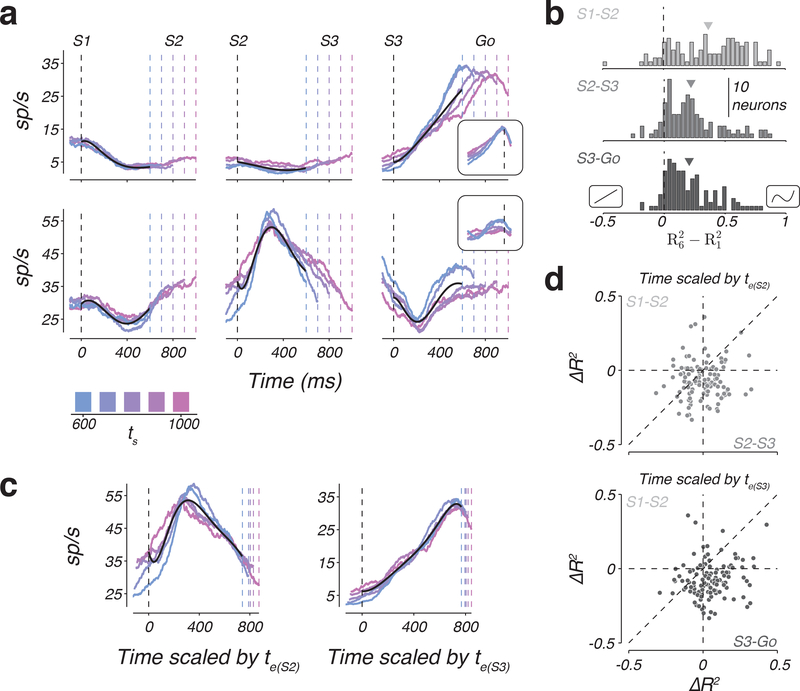
Figure 4. Temporal scaling of non-monotonic firing rates across individual DMFC neurons.

a) Firing rates of two example neurons (rows) as a function of task epoch (columns) for different values of t_s (colors). Black lines are the fit of a 6th order polynomial to the first 600 ms of each epoch and neuron. From left to right, firing rates were aligned to S1, S2, and S3 flashes, respectively (black dashed line). Colored dashed lines represent the time of the subsequent flash. Insets: firing rates aligned to Go (black dashed line). b) Histograms of the difference in the fraction of variance explained, R², between the 6th and 1st order polynomial fit to the data. Negative and positive values correspond to neurons that favored the 1st and 6th order polynomial, respectively. Insets on the negative and positive sides of the abscissa illustrate example 1st and 6th order polynomials. Arrows indicate the mean of the distributions. Different gray levels correspond to different task epochs. c) Example scaled temporal responses. Left: firing rate of the second neuron in panel a during the S2-S3 epoch, temporally scaled by the animals’ estimate in the S2-S3 epoch. The estimate was inferred from the model fits to the behavior. Right: firing rate profile for the S3-Go epoch of the first neuron in panel a temporally scaled by the animals’ estimate in the S3-Go epoch. Black lines show the 6th order polynomial that best fit the scaled data. Dashed lines as in panel a, but appropriately scaled. d) Scatter plot showing the change of explanatory power (ΔR²) of the 6th order polynomial fit to the scaled versus unscaled data across neurons. Top: ΔR² in the S2-S3 epoch compared to the S1-S2 epoch. Bottom: ΔR² in the S3-Go epoch compared to the S1-S2 epoch. Vertical and horizontal dashed lines indicate ΔR² = 0 and the diagonal in the unity line. See also Supplementary Figures 2 and 3.