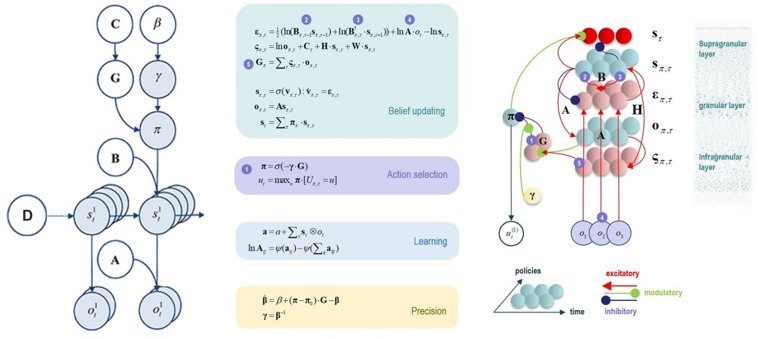
FIGURE 2.

This figure illustrates the mathematical framework of active inference and associated neural process theory used in the simulations described in this paper. (Left) Illustration of the Markov decision process formulation of active inference. The generative model is here depicted graphically, such that arrows indicate dependencies between variables. Here observations (o) depend on hidden states (s), as specified by the A matrix, and those states depend on both previous states (as specified by the B matrix, or the initial states specified by the D matrix) and the policies (π) selected by the agent. The probability of selecting a particular policy in turn depends on the expected free energy (G) of each policy with respect to the prior preferences (C) of the agent. The degree to which expected free energy influences policy selection is also modulated by a prior policy precision parameter (γ), which is in turn dependent on beta (β) – where higher values of beta promote more randomness in policy selection (i.e., less influence of the differences in expected free energy across policies). (Middle/Right) The differential equations in the middle panel approximate Bayesian belief updating within the graphical model depicted on the left via a gradient descent on free energy (F). The right panel also illustrates the proposed neural basis by which neurons making up cortical columns could implement these equations. The equations have been expressed in terms of two types of prediction errors. State prediction errors (ε) signal the difference between the (logarithms of) expected states (s) under each policy and time point and the corresponding predictions based upon outcomes/observations (A matrix) and the (preceding and subsequent) hidden states (B matrix, and, although not written, the D matrix for the initial hidden states at the first time point). These represent prior and likelihood terms, respectively – also marked as messages 2, 3, and 4, which are depicted as being passed between neural populations (colored balls) via particular synaptic connections in the right panel (note: the dot notation indicates transposed matrix multiplication within the update equations for prediction errors). These (prediction error) signals drive depolarization (v) in those neurons encoding hidden states (s), where the probability distribution over hidden states is then obtained via a softmax (normalized exponential) function (σ). Outcome prediction errors (σ) instead signal the difference between the (logarithms of) expected observations (o) and those predicted under prior preferences (C). This term additionally considers the expected ambiguity or conditional entropy (H) between states and outcomes as well as a novelty term (W) reflecting the degree to which beliefs about how states generate outcomes would change upon observing different possible state-outcome mappings (computed from the A matrix). This prediction error is weighted by the expected observations to evaluate the expected free energy (G) for each policy (π), conveyed via message 5. These policy-specific free energies are then integrated to give the policy expectations via a softmax function, conveyed through message 1. Actions at each time point (u) are then chosen out of the possible actions under each policy (U) weighted by the value (negative expected free energy) of each policy. In our simulations, the agent learned associations between hidden states and observations (A) via a process in which counts were accumulated (a) reflecting the number of times the agent observed a particular outcome when she believed that she occupied each possible hidden state. Although not displayed explicitly, learning prior expectations over initial hidden states (D) is similarly accomplished via accumulation of concentration parameters (d). These prior expectations reflect counts of how many times the agent believes she previously occupied each possible initial state. Concentration parameters are converted into expected log probabilities using digamma functions (ψ). As already stated, the right panel illustrates a possible neural implementation of the update equations in the middle panel. In this implementation, probability estimates have been associated with neuronal populations that are arranged to reproduce known intrinsic (within cortical area) connections. Red connections are excitatory, blue connections are inhibitory, and green connections are modulatory (i.e., involve a multiplication or weighting). These connections mediate the message passing associated with the equations in the middle panel. Cyan units correspond to expectations about hidden states and (future) outcomes under each policy, while red states indicate their Bayesian model averages (i.e., a “best guess” based on the average of the probability estimates for the states and outcomes across policies, weighted by the probability estimates for their associated policies). Pink units correspond to (state and outcome) prediction errors that are averaged to evaluate expected free energy and subsequent policy expectations (in the lower part of the network). This (neural) network formulation of belief updating means that connection strengths correspond to the parameters of the generative model described in the text. Learning then corresponds to changes in the synaptic connection strengths. Only exemplar connections are shown to avoid visual clutter. Furthermore, we have just shown neuronal populations encoding hidden states under two policies over three time points (i.e., two transitions), whereas in the task described in this paper there are greater number of allowable policies. For more information regarding the mathematics and processes illustrated in this figure, see Friston et al. (2016, 2017a,b,c).