Figure 4. Deletion of Vangl2 decreases actin treadmilling.

(A) Representative images of growth cones from control and Vangl2 cKO neurons expressing GFP and actin-mEos2. Images show the growth cone filled with GFP (left) and the trajectories of single actin-mEos2 molecules (in black) recorded over a 3 min period at 2 Hz (right). Insets show higher-magnification examples of the variability in individual trajectories. Scale bar, 5 µm. (B, C) Distribution of actin-mEos2 molecules α values in control and Vangl2 cKO neurons. n = 184–440 trajectories, 6–7 neurons. (D) Frequency distribution of directed, Brownian and confined trajectories of actin-mEos2 molecules in control and Vangl2 cKO neurons plated on Ncad-Fc substrates. (E) Speed of retrograde actin flow as extracted from the directed trajectories in controls and Vangl2 cKO neurons. n = 73–79 trajectories, 6–7 neurons. n = 8 sister cultures (DIV3) from eight different mice. (F, G) Quantification of the speed and lifetime of EB3-GFP particles in control and Vangl2 cKO neurons. n = 18–19 neurons. Data are presented as box-and-whisker plots (min/max) based on three independent experiments; *p<0.05, **p<0.01 by the Mann-Whitney test (D, E).

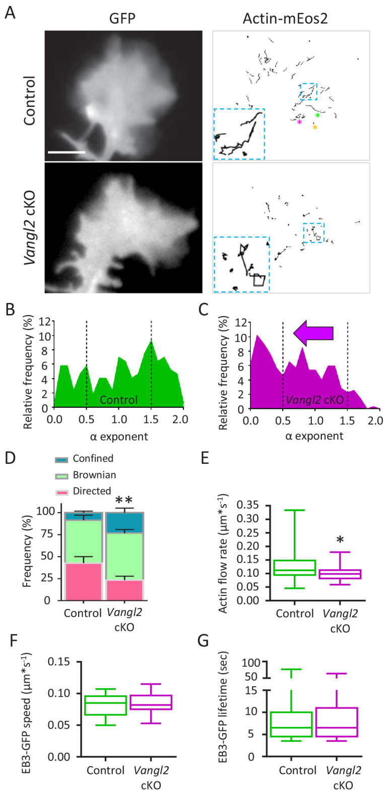
Figure 4—figure supplement 1. SptPALM is an accurate method for the analysis of F-actin flow in growth cones.

(A) Distribution of the actin-mEos2 trajectory length shows a median trajectory (dotted line) length of 9 frames for both genotypes. (B) Distribution of α exponents obtained by fitting the MSD of purely diffusive simulated actin trajectories (no flow). As expected, the distribution is centered around 1, and 90% of the population lies in the interval 0.5 < α <1.5. According to these results, the thresholds for confined and directed motions were set to α = 0.5 and 1.5, respectively. (C, D) Schematic representations of trajectories according to their α values (C), and representation of typical curves obtained for each trajectory type after fitting the MSD values by the power law 4Dtα (D). (E, F) Representative growth cone from a control neuron expressing GFP and actin-mEos2 and plated on Poly-L-lysine (PLL) coated glass. Images show the GFP signal (left, white) and the trajectories of single actin-mEos2 molecules in the peripheral region recorded over a 3 min period at 2 Hz (right, black). The inset shows directed trajectories at higher magnification. Red dotted lines show a region used for kymograph analysis. Scale bar, 5 µm. (G, H) Average surface area and migration speed of growth cones from control neurons plated on PLL or N-cadherin. (I) Representative kymograph from the peripheral region of a control growth cone plated on PLL, representing actin-mEos2 displacement as a function of time. (J) Speed of retrograde actin flow as extracted from the directed trajectories in control neurons (green, n = 929 trajectories, six growth cones) or by kymograph analysis (purple, n = 277 trajectories, six growth cones). (K) Distribution of the values of the exponent α obtained after fitting the MSD of single actin-mEos2 trajectories, for control neurons plated on PLL (n = 929 trajectories from six neurons). (L) Western blots and quantifications showing the expression of G- and F-actin in both control and Vangl2 cKO mice. N = 8 sister cultures (DIV3) from eight different mice; *p<0.05 and ****p>0.0001 by Student’s t-test (H) or by the Mann-Whitney test (G).

Figure 4—figure supplement 2. Theoretical prediction of the mechanical coupling between the actin flow and transmembrane adhesion.

(A) Example of a computer simulation showing the trajectory of a single actin molecule in a virtual growth cone (whole duration 160 s, time increment 50 ms). Actin alternates between periods of fast free diffusion when it is monomeric G-actin (blue arrow), and slow rearward flow when it is assembled in the filamentous F-actin network (red arrows). Polymerization occurs preferentially at the peripheral edge of the growth cone, and depolymerization at the base. (B) Color-coded image of a virtual growth cone showing the maximal intensity projection of 400 actin molecules, integrated over time. The fluorescence-like image is generated by representing each molecule as a Gaussian intensity profile, accumulated for 250 ms. Note intense tracks corresponding to the persistent radial motion of actin molecules incorporated in the filamentous fraction (green), and a weak blur corresponding to randomly moving actin monomers (violet). (C) Three examples of the mean square displacement (MSD) over time, for three representative trajectories of each type of motion (directed, Brownian, and confined). Inset images show individual simulated actin trajectories for different values of the coupling strength to transmembrane adhesion. Molecules are made fluorescent for short durations (<a few seconds), tightly corresponding to the experimental values measured for actin-mEos2. Only trajectories lasting more than seven frames are selected. The data were fitted by the power function 4Dtα, where D is a diffusion coefficient, and an α exponent between 0 and 2. The α-values are indicated in the graphs (correlation coefficient r > 0.95 in all cases). (D) Histograms of the distribution of α exponents for different levels of coupling strength (n = 28 and 51 trajectories, respectively) and flow velocity. (E, F) Relationship between the fraction of directed trajectories and the coupling strength or the actin velocity, respectively (n = 28–51 trajectories for each condition).