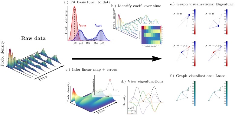
Fig 1. Illustration of Dynamic Distribution Decomposition workflow.

(a.) Gaussian mixture models as basis functions: single-cell profiles from each time point are fitted to a basis of Gaussian mixture model, two distributions shown in red and blue; (b.) identification of the coefficients c(t) at each time point, t = t₁, …, t_R; (c.) the Perron–Frobenius matrix P enables us us to infer the likely state for all time points and generate errors ε₁, …, ε_R; (d.) examination of the eigenfunctions in low dimensions; or in high dimensions (e.) using graphical visualisations; and (f.) a Lasso regularisation can reveal sparse structure.