. 2019 Dec 19;8:e50576. doi: 10.7554/eLife.50576

Figure 7. Estimate of the free-energy cost associated with the membrane deformation caused by all-inward GltPh, from direct potential-of-mean-force calculations.

(A) Simulated membrane deformation, in the absence of the protein, induced by application of the Multi-Map method in combination with umbrella sampling, for a coarse-grained POPC lipid bilayer at 298 K. The figure shows three deflection maps analogous to those shown in Figure 2A, that is calculated from trajectory data by averaging the Z coordinate of the bilayer mid-plane across the range of X and Y encompassed by the simulation box. The deflection maps shown correspond to three individual umbrella-sampling windows used in this free-energy calculation, differing in the amplitude of the perturbation that is induced in each case. Other trajectories/windows sample deformation amplitudes that are smaller or larger than those represented in the figure, that is, smaller or larger values of the Multi-Map variable. Each map reflects an average of 18 independent simulations of 1 μs each. (B) Potential-of-mean-force (PMF) curve for the morphological perturbation depicted in panel (A), as a function of the Multi-Map variable, that is, as a function of an increasing deformation amplitude. The free-energy values for the three configurations represented in panel (A) are indicated. PMF curves are also shown for two additional calculations based on umbrella-sampling simulations under an applied membrane tension, for the values indicated. Each of these PMF curves is an average of 18 independent calculations, each sampling 1 μs per window. Error bars for each curve average to about 0.6 kcal/mol.

Figure 7.

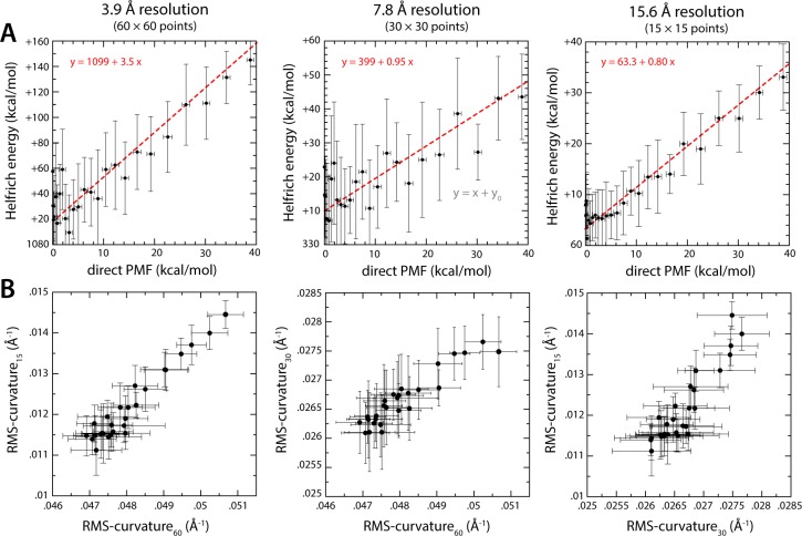
Figure 7—figure supplement 1. Comparison of membrane-bending free-energy values calculated with the Multi-Map method and with the Helfrich-Canham theory, for the same ensembles of molecular configurations.

Figure 7—figure supplement 1.

(A) The PMF curves shown in Figure 7 are correlated with energy profiles calculated with the Helfrich-Canham equation. Calculation of the latter requires two inputs: the assumed bending modulus kc and the membrane curvature distribution across the X-Y plane, c(x, y). For each of the umbrella-sampling windows used in the PMF calculation (18 trajectories × 1 μs), that is for each value of the progress variable ξ, we evaluate this curvature distribution from analysis of the average mid-plane of the membrane; specifically, maps such as those shown in Figure 7A were interpolated with cubic splines and differentiated with respect to coordinates x and y to obtain the corresponding local curvature maps, c(x, y). The elastic energy for each value of ξ was then calculated by integrating the Helfrich-Canham energy density [0.5 kc c2(x, y)] over the area of the membrane. The three plots in panel (A) describe Helfrich-Canham calculations that use the same value of kc, namely 18 kcal/mol (Fiorin et al., 2019), but differ in the level of resolution used to quantify c(x, y), as indicated. Linear regressions of the data in each case (using points up to ~100 kcal/mol – dashed red lines) show that the Helfrich-Canham energies can be much larger, similar or somewhat smaller that the PMF values depending on the resolution used for this curvature evaluation. (B) Comparison of curvature evaluations carried out at different resolutions. Specifically, for each umbrella-sampling window we compute the root-mean-squared curvature across the whole bilayer plane and contrast different resolutions. Despite extensive simulation time, that is 18 trajectories × 1 μs per window, the evaluation of the local membrane curvature is prone to large statistical errors (which propagate to the energy calculations) and ill-defined averages for moderate to low curvature values. By contrast, the PMFs curves shown in Figure 7 approximately converge after 1 μs of sampling per window. In our view, these ambiguities in the definition of membrane curvature and the appropriate value of the bending modulus highlight the merits of direct PMF calculations such as those shown in Figure 7.