Automatic kidney segmentation in ultrasound images using subsequent boundary distance regression and pixelwise classification networks

Abstract

It remains challenging to automatically segment kidneys in clinical ultrasound (US) images due to the kidneys’ varied shapes and image intensity distributions, although semi-automatic methods have achieved promising performance. In this study, we propose subsequent boundary distance regression and pixel classification networks to segment the kidneys automatically. Particularly, we first use deep neural networks pre-trained for classification of natural images to extract high-level image features from US images. These features are used as input to learn kidney boundary distance maps using a boundary distance regression network and the predicted boundary distance maps are classified as kidney pixels or non-kidney pixels using a pixelwise classification network in an end-to-end learning fashion. We also adopted a data-augmentation method based on kidney shape registration to generate enriched training data from a small number of US images with manually segmented kidney labels. Experimental results have demonstrated that our method could automatically segment the kidney with promising performance, significantly better than deep learning-based pixel classification networks.

1. INTRODUCTION

Ultrasound (US) imaging has been widely used to aid diagnosis and prognosis of acute and chronic kidney diseases (Ozmen et al., 2010; Pulido et al., 2014). In particular, anatomic characteristics derived from US imaging, such as renal elasticity, are associated with kidney function (Meola et al., 2016) and lower renal parenchymal area measured on US images is associated with increased risk of end-stage renal disease (ESRD) in boys with posterior urethral valves (Pulido et al., 2014). Imaging features computed from US data using deep convolutional neural networks (CNNs) improved the classification of children with congenital abnormalities of the kidney and urinary tract (CAKUT) and controls (Zheng et al., 2019; Zheng et al., 2018a). The computation of these anatomic measures typically involves manual or semi-automatic segmentation of kidneys in US images, which increases inter-operator variability, reduces reliability, and limits utility in clinical medicine. Automatic and reliable segmentation of the kidney from US imaging data would improve precision and its application in many different clinical conditions including congenital renal disease, renal mass detection, and kidney stones.

Since manual segmentation of the kidney is time consuming, labor-intensive, and highly prone to intra- and inter-operator variability, semi-automatic and interactive segmentation methods have been developed (Torres et al., 2018). Particularly, an interactive tool has been developed for detecting and segmenting the kidney in 3D US images (Ardon et al., 2015). A semi-automatic segmentation framework based on both texture and shape priors has been proposed for segmenting the kidney from noisy US images (Jun et al., 2005). A graph-cuts method has been proposed to segment the kidney in US images by integrating image intensity information and texture information (Zheng et al., 2018b). A variety of methods have been proposed to segment the kidney based on active shape models and statistical shape models (Ardon et al., 2015; Cerrolaza et al., 2016; Cerrolaza et al., 2014; Martín-Fernández and Alberola-López, 2005; Mendoza et al., 2013). Random forests have been adopted in a semi-automatic segmentation method to segment the kidney (Sharma et al., 2015). An automated approach has been developed for kidney segmentation in three-dimensional US Images by initializing and evolving a level-set function through shape-to-volume registration and statistical shape modeling (Marsousi et al., 2017). Although a variety of strategies have been adopted in these kidney segmentation methods, most of them solve the kidney segmentation problem as a boundary detection problem.

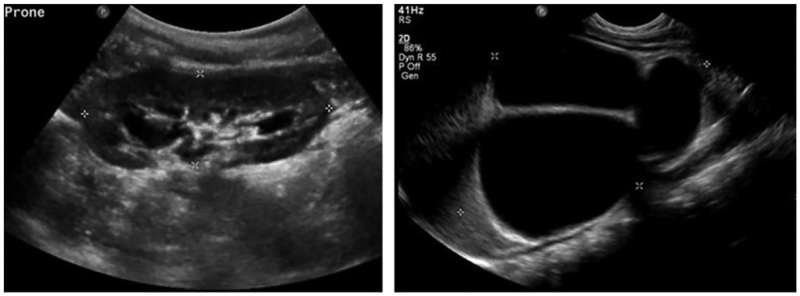
Deep CNNs have demonstrated excellent performance in a variety of image segmentation problems, including semantic segmentation of natural images (Badrinarayanan et al., 2017; Chen et al., 2018a; Chen et al., 2018b; Long et al., 2015; Zhao et al., 2017) and medical image segmentation (Li et al., 2019a; Li et al., 2018; Li et al., 2019b; Men et al.; Ronneberger et al., 2015; Zhao et al., 2016; Zhao et al., 2018a, b). In these studies, the image segmentation problems are solved as pixelwise or voxelwise pattern classification problems. Recently, several methods have been proposed to automatically segment the kidney from medical imaging data to generate kidney masks using deep CNNs. In particular, Unet networks have been adopted to segment the kidney (Jackson et al., 2018; Ravishankar et al., 2017; Sharma et al., 2017). In these pattern classification-based kidney segmentation methods, all pixels/voxels within the kidney have the same kidney classification labels. Such a strategy might be sensitive to large variability of the kidneys in both appearance and shape in US images. As shown in Fig. 1, kidneys may have varied shapes and heterogeneous appearances in US images. The shape and appearance variability of kidneys, in conjunction with inherent speckle noise of US images, may degrade performance of the pixelwise pattern classification based kidney segmentation methods (Noble and Boukerroui, 2006).

Fig. 1.

Kidneys in US images may have varied shapes and the kidney pixels typically have heterogeneous intensities and textures.

On the other hand, several recent studies have demonstrated that pixelwise pattern classification based image segmentation methods could achieve improved image segmentation performance by incorporating boundary detection as an auxiliary task in both natural image segmentation (Bertasius et al., 2015; Chen et al., 2016) and medical image segmentation (Chen et al., 2017; Tang et al., 2018). However, the performance of these methods is hinged on their image pixelwise classification component as the boundary detection serves as an auxiliary task for refining edges of the pixelwise segmentation results.

Inspired by the excellent performance of the boundary detection-based kidney segmentation methods, we develop a fully automatic, end-to-end deep learning method to subsequently learn kidney boundaries and pixelwise kidney masks from a set of manually labeled US images. Instead of directly distinguishing kidney pixels from non-kidney ones in a pattern classification setting, we learn CNNs in a regression setting to detect kidney boundaries that are modeled as boundary distance maps. From the learned boundary distance maps, we learn pixelwise kidney masks by optimizing their overlap with the manual kidney segmentation labels. To augment the training dataset, we adopt a kidney shape-based image registration method to generate more training samples. Our deep CNNs are built upon an image segmentation network architecture derived from DeepLab (Chen et al., 2018b) so that existing image classification/segmentation models could be reused as a starting point of the kidney image segmentation in a transfer learning framework to speed up the model training and improve the performance of the kidney image segmentation. We have evaluated the proposed method for segmenting the kidney based on 289 clinical US images. Experimental results have demonstrated that the proposed method could achieve promising segmentation performance and outperformed alternative state-of-the-art deep learning based image segmentation methods, including FCNN (Long et al., 2015), Deeplab (Chen et al., 2018b), SegNet (Badrinarayanan et al., 2017), Unet (Ronneberger et al., 2015), PSPnet (Zhao et al., 2017), and DeeplabV3+(Chen et al., 2018a). Our image segmentation method is built on a kidney boundary detection network presented at ISBI 2019 (Yin et al., 2019), enhanced by a novel data augmentation method to improve the segmentation results. The present study also investigates how different parameter settings and training strategies affect the segmentation performance and compares our method with more alternative deep learning segmentation methods, including a multi-task learning network.

2. METHODS AND MATERIALS

2.1. Imaging Data

We used 289 US images to train and evaluate the proposed method. The images were collected from 152 subjects (male: 106; age: 83.3 ± 161.6 days). Among these subjects, 137 had bilateral kidney images, 4 had left kidney images, and 11 had right kidney images. All the images were in sagittal view, collected for routine clinical care using Philips, Siemens, or General Electric ultrasound scanners with an abdominal transducer. All the images had 1024×768 pixels with pixel size ranging from 0.08×0.08mm² to 0.12×0.12mm². All identifying information was removed from the images. The work described has been carried out in accordance with the Declaration of Helsinki. The study has been reviewed and approved by the institutional review board at the Children’s Hospital of Philadelphia (CHOP). Representative kidney US images are shown in Fig. 1.

The images were manually segmented by two urologists who are experts in interpreting clinical ultrasounds. For accessing the inter-rater reliability, 20 images were randomly selected, including 3 with boundary cut. In terms of Dice index, the overall inter-rater variability was 0.95±0.02, the inter-rater variability on the images with boundary cut was 0.92±0.03, and the inter-rater variability on the remaining images was 0.96±0.01.

All the images were resized to have the same size of 321×321, and their image intensities were linearly scaled to [0,255]. We randomly selected 105 images as training data and 20 images as validation data in the present study to train deep learning-based kidney segmentation models. The remaining 164 US images were used to evaluate the proposed method.

2.2. Deep CNN Networks for Kidney Image Segmentation

The kidney image segmentation method is built upon deep CNNs to subsequently detect kidney boundaries and kidney masks in an end-to-end learning fashion. As illustrated in Fig. 2, the kidney image segmentation model consists of a transfer learning network, a boundary distance regression network, and a kidney pixelwise classification network. The transfer learning network is built upon a general image classification network to reuse an image classification model as a starting point for learning high level image features from US images, the boundary distance regression network learns kidney boundaries modeled as distance maps of the kidney boundaries, and the kidney boundary distance maps are finally used as input to the kidney pixelwise classification network to generate kidney segmentation masks.

Fig. 2.

Transfer learning network, and subsequent boundary distance regression and pixel classification networks for fully automatic kidney segmentation in US images. The boundary detection network (Bnet) is trained using a distance loss function and the end-to-end subsequent segmentation network is trained by combining the distance loss function and a softmax loss function.

The kidney distance regression network and the kidney pixelwise classification network are trained based on augmented training data that are generated using a kidney shape-based image registration method. The network architecture and the data augmentation methods are described in following sections.

2.2.1. Transfer learning network for extracting high level image features from US images

Instead of directly building an image segmentation network on raw US images, we adopt a transfer learning strategy to extract informative image features from US images as a starting point for learning high level image features from US images. Particularly, we extract features from US images by utilizing a general image classification network, namely VGG16, which achieves 92.7% top-5 test-accuracy in ImageNet [34].

As illustrated in Fig. 3, the VGG16 network consists of 16 convolutional (conv) layers with a receptive field of 3×3. The stack of convolutional layers is followed by 3 fully-connected (FC) layers: each of the first two has 4096 channels and the third performs 1000-way classification. The final layer is a softmax layer. In our experiments, we fine-tuned the model weights of Imagenet-pretrained VGG16 network to adapt them to the boundary distance regression network.

Fig. 3.

The architecture of theVGG16 model.

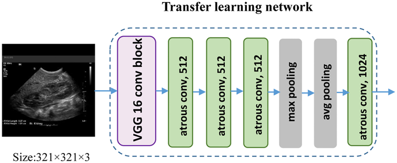
On the other hand, we follow the Deeplab architecture by applying the atrous convolutions (Chen et al., 2018b) to compute denser image feature representations. Particularly, the Deeplab image segmentation model replaced the last 3 convolutional layers and FC layers of VGG16 with into 4 atrous convolutional layers and 2 convolutional classification layers. As illustrated in Fig. 4, we discarded the 2 convolutional classification layers to adapt the architecture to the boundary distance regression network.

Fig. 4.

The transfer learning architecture of the Deeplab model (Chen et al., 2018b). We extracted the pretrained feature maps from the exiting Deeplab model.

2.2.2. Boundary distance regression network for fully automatic kidney segmentation in ultrasound images

We develop a boundary distance regression network for fully automatic kidney segmentation in ultrasound images, instead of learning a pixelwise classification network directly from the US image features, because the heterogenous kidney appearances in US images make it difficult to directly classify pixels as kidney or background pixels.

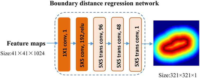
The boundary distance regression network is built in a regression framework, consisting of two parts: a projection part that produces boundary feature maps S₀ and a high-resolution reconstruction part that upsamples the feature maps to obtain the kidney distance maps at the same spatial resolution of the input images as illustrated in Fig. 5. The projection part is built on two convolutional layers, and the reconstruction part is built on deconvolution (transposed convolution) layers. The output of the ith deconvolution operation S_i is defined as

$$S_i=\mathit{\text{max}}\left(0,W_i\otimes S_{i-1}+B_i\right),$$ (1)

where W_i is deconvolution filters with size f_i × f_i, and B_i is a bias vector, and ⊗ is deconvolution operator. The upsampling deconvolution layers double the spatial dimension of their input feature maps, and therefore 3 upsampling deconvolution layers are adopted in the kidney boundary distance regression network to learn the kidney boundary in the input image space. In our experiments, the numbers of input feature maps of the upsampling deconvolution layers were empirically set to 3 times of 64, 32, 16 respectively, and the filter size f_i was empirically set to 5.

Fig. 5.

Network architecture of the boundary distance regression network.

We solve the kidney boundary detection problem in a regression framework to learn distance from the kidney boundary for every pixel of the input US images. The kidney boundary detection problem could be potentially solved in an end-to-end classification framework (Xie and Tu, 2015). However, the number of the kidney boundary pixels is much smaller than the number of non-boundary pixels in US kidney images. Such unbalanced boundary and non-boundary pixels make it difficult to learn an accuracy classification model. Therefore, we model the kidney boundary detection as a distance map learning problem.

Given an input US image I with its kidney boundary, we compute the distance to the kidney boundary for every pixel P_i ∈ I of the input image and obtain a normalized kidney distance map of the same size of the input image using potential function as following:

$$d\left(P_i\right)=\mathit{\text{exp}}\left(-\lambda D_i\right),$$ (2)

with $D_i={\text{min}}_{b_j\in b}\text{dist}\left(P_i,b_j\right)$ is the minimal Euclidean distance of pixel P_i to the kidney boundary pixels b= {b_j}_j∈j, and λ is a parameter. As illustrated in Fig. 6, at the kidney boundary pixels the normalized exponential kidney distance equals to 1. In this study, the kidney boundary is detected by learning the normalized kidney distance map.

Fig. 6.

An example kidney US image and kidney boundary (a), its boundary distance map (b), and its normalized potential distance map with λ = 1 (c). The colorbar of (c) is in log scale.

To learn the normalized kidney boundary distance map, we train the boundary detection network by minimizing a distance loss function L_d, defined as,

$$L_d={\sum }_{P_i\in I}{\Vert \phi \left(P_i\right)-d\left(P_i\right)\Vert }^2,$$ (3)

where φ(P_i) is the predicted distance and d(P_i) is the ground truth distance to the kidney boundary at pixel P_i. Once we obtain the predicted distance for every pixel of a US image to be segmented, we can obtain a boundary binary map with a threshold e^−λ.

To obtain a smooth closed contour of the kidney boundary, we construct a minimum spanning tree of all predicted kidney boundary pixels. Particularly, we first construct an undirected graph of all predicted kidney boundary pixels, each pair of which are connected with a weight of their Euclidean distance. Then, a minimum spanning tree T is obtained using Kruskal’s algorithm (Kruskal, 1956). Finally, the max path of the minimum spanning tree T is obtained as a close contour of the kidney boundary and a binary mask of the kidney is subsequently obtained. To reduce the complexity of finding a minimum spanning tree, we apply binary image skeleton morphology operator to the binary kidney boundary image in order to obtain a skeleton binary map, then apply the minimum spanning tree algorithm to the skeleton binary map, and finally use poly2mask to compute a binary mask based on a polygon obtained by the minimum spanning tree algorithm. We refer to the boundary distance regression network followed by post-processing for segmenting kidneys as a boundary detection network (Bnet) hereafter as shown in Fig. 2. Table 1 highlights differences between the boundary detection network and the end-to-end learning of subsequent boundary distance regression and pixelwise classification networks.

Table 1.

Differences between the boundary detection network and the end-to-end learning of subsequent boundary distance regression and pixelwise classification networks.

	Transfer learning network	Boundary distance regression network	Post processing	Pixelwise classification network	Distance loss function	Softmax loss function
Boundary Detection Network	✓	✓	✓		✓
End-to-end learning of subsequent segmentation networks	✓	✓		✓	✓	✓

2.2.3. Subsequent boundary distance regression and pixelwise classification networks for fully automatic kidney segmentation in ultrasound images

The minimum spanning tree post-processing method could obtain promising boundary detection results for most US kidney images. However, it fails if the predicted boundary distance maps are far from perfect. To obtain robust kidney segmentation performance, we propose to learn pixelwise kidney masks from the predicted kidney distance maps.

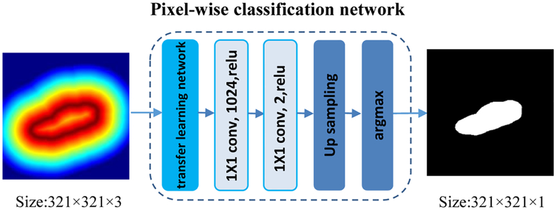
As illustrated in Fig. 7, the kidney pixelwise classification network is built upon a semantic image segmentation network, namely Deeplab image segmentation network. The input to the kidney pixel classification network is an image with 3 channels, each being the output of the predicted kidney boundary map. The final decision for class labels is then made by applying 2-channel classification softmax layer to the extracted class feature maps $f_{\left(c,P_i\right)}(c=0,1)$ (c=0,1) based on cross-entropy loss function. We also adopt the pre-trained VGG16 model to initialize the pixelwise classification network parameters.

Fig. 7.

Architecture of the kidney pixel classification network.

To train the kidney boundary distance regression and pixelwise classification networks in an end-to-end fashion, loss functions of the kidney boundary distance regression network and the kidney pixelwise classification network are combined as a multi-loss function

$$L_m=\left(1-\frac{\tau }{N}\right)L_d+\frac{\tau }{N}\gamma L_S,$$ (5)

where N is the number of total iterative training steps, τ is an index of the training iteration step, and γ is a parameter to make L_d and L_s to have the same magnitude and to be determined empirically. The multi-loss function puts more weight on the kidney boundary distance regression cost function in the early stage of the network training and then shifts to the kidney pixel classification cost function in the late stage of the network training. The kidney pixelwise classification network’s output is treated as the overall segmentation result.

2.3. Data augmentation based on kidney shape registration

To build a robust kidney segmentation model, we augment the training data using a non-rigid image registration method (Bookstein, 1989). Particularly, in order to generate training US kidney images with varied kidney shapes and appearances, we register each training image to all other training images based on thin-plate splines transformation (TPS) (Bookstein, 1989) as following.

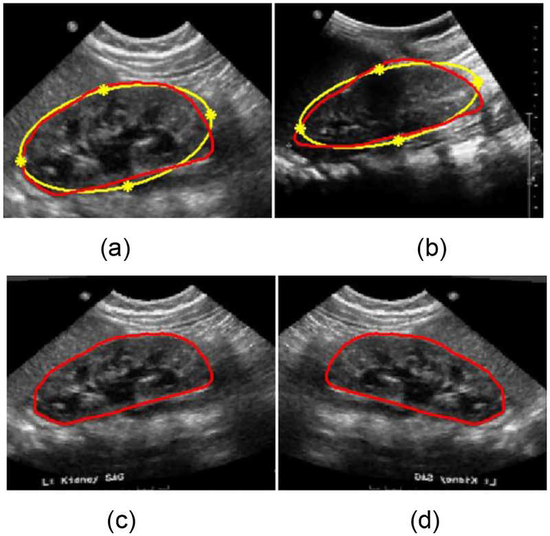
Given two US kidney images with kidney boundaries, we register one image (moving image M) to the other image (fixed image F), in order to generate a deformed moving image in the fixed image space. First, the kidney boundary is approximately modeled as an ellipse as shown in Fig. 8. Then, ellipse vertexes of the kidney are identified as 4 corresponding landmark points across kidneys, and the landmark points of the fixed and moving images are denoted by Z_M = [x_M y_M]^T ∈ R^2×4 and Z_F= [x_F y_F]^T ∈ R^2×4 respectively. Base on the corresponding landmark points, a TPS operation W is computed to register the moving image M to the fixed image F, defined as:

$$\mathit{W}={\left[\begin{array}{cc}R& P^T\\ P& 0^{3\times 3}\end{array}\right]}^{-1}\left[\begin{array}{c}{Z}_M^T\\ 0^{3\times 2}\end{array}\right],$$ (6)

where $P={\left[\begin{array}{ll}{I}^{4\times 1}\hfill & Z_M^T\hfill \end{array}\right]}^T\in R^{3\times 4}$ is the homogeneous coordinates of Z_M, and R is a symmetric matrix with elements r_i,j = ϕ(KZ_M – Z_MK₂). Based on the estimated TPS transformation, a warped moving image could be generated. We use a nearest neighbor interpolation method to warp the moving image. In addition to the image registration-based data augmentation, we also flip the training images left to right. Given n training images, we can obtain 2n(n − 1) + n augmented training images with kidney boundaries.

Fig. 8.

Data-augmentation based on TPS transformation and flipping. (a) is a moving image, (b) is a fixed image, (c) is the registered image and (d) is the flipped registered image. The kidney shape denoted by the red curve is approximately modeled as an ellipse denoted by the yellow curves. The yellow stars denote the landmark points of the TPS transformation.

2.4. Implementation and Evaluation of the proposed method

The proposed networks were implemented based on Python 3.7.0 and TensorFlow r1.11. We used a mini-batch of 20 images to train the deep neural networks. The maximum number of iteration steps was set to 20000. The deep learning models were trained on a GeForce GTX 980 Ti graphics processing unit (GPU). The deep networks were optimized using Adam stochastic optimization (Boyd and Vandenberghe, 2004) with the learning rate of 10⁻⁴. Besides the parameters of transfer learning network, the filters of the boundary regression network were initialized with random normal initializer with the mean 0 and standard deviation 0.001. The biases of the boundary regression network were initialized with constant 0. In the subsequent kidney boundary detection and pixel classification network, γ was empirically set to 1 to make the kidney boundary regression and pixel classification loss functions to have similar magnitudes. The minimum spanning tree algorithm were implemented based on Networkx python library (https://networkx.github.io/documentation/networkx-1.10/overview.html).

Ablation studies were carried out to evaluate how different components of the proposed method affect the segmentation performance. We first trained the kidney boundary detection network using following 3 different strategies, including training from scratch without data augmentation (named “random+noaug”), transfer learning without data augmentation (named “finetune+noaug”), and transfer-learning with data augmentation (named “finetune+aug”). Particularly, for the training from scratch we adopted “Xavier” initialization method that has been widely adopted in natural image classification and segmentation studies (Glorot and Bengio, 2010). Particularly, we initialized the biases to be 0 and filters to follow a uniform distribution. The training images’ normalized kidney boundary distance maps were obtained with λ = 1. Outputs of the kidney boundary detection network were post-processed using morphological operations and minimum spanning tree algorithm in order to obtain kidney masks.

Second, we trained and compared kidney boundary detection networks based on augmented training data and transfer-learning initialization with their normalized kidney distance maps obtained with different values of λ, including 0.01, 0.1, 1, and 10. We also trained a kidney boundary detection network in a classification setting. Particularly, the classification-based kidney boundary detection network had the same network architecture as the regression-based kidney boundary detection network, except that its loss function was a softmax cross-entropy loss to directly predict the kidney boundary pixels. Outputs of the kidney boundary detection network were also post-processed using the morphological operations and minimum spanning tree algorithm in order to obtain kidney masks.

Third, we trained and compared kidney boundary detection networks with 6 state-of-the-art pixel classification based image segmentation deep neural networks, namely FCNN (Long et al., 2015), Deeplab (Chen et al., 2018b), SegNet (Badrinarayanan et al., 2017), Unet (Ronneberger et al., 2015), PSPnet (Zhao et al., 2017), and DeeplabV3+(Chen et al., 2018a). These networks also adopted encoding part of the VGG16, the same one as adopted in our method. The comparisons were based on both the training data without augmentation and the augmented training data. Segmentation performance of all the methods under comparison was measured using Dice index, mean distance (MD), Jaccard, Precision, Sensitivity, ASSD as defined in (Hao et al., 2014; Zheng et al., 2018c). The units of MD and ASSD were pixels. The segmentation performance measures of testing images obtained by different segmentation networks were statistically compared using Wilcoxon signed-rank tests (Woolson, 2008).

We also used 5-fold cross-validation to compare our method with PSPnet and Deeplabv3+ that had the best performance as pixelwise classification networks. In each cross-validation experiment, all the training images were augmented using the proposed data-augmentation method. The number of training iteration steps was set to 30000 in the cross-validation experiments.

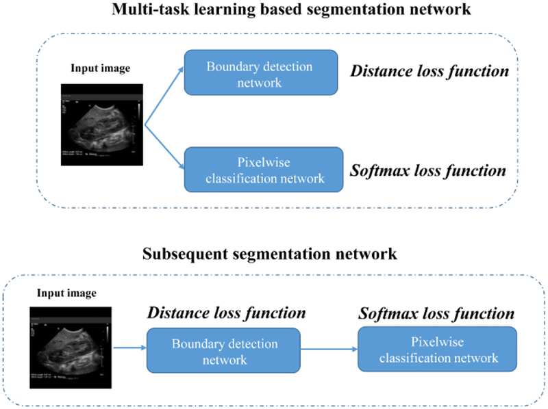
We compared the proposed subsequent boundary distance regression and pixelwise classification networks with the kidney boundary detection network. We trained the subsequent boundary distance regression and pixelwise classification network based on the augmented training data and transfer-learning initialization. We also compared the proposed framework with a multi-task learning based segmentation network to jointly estimate the kidney distance maps and classify the kidney pixels, as illustrated by Fig. 1. The multi-task learning based segmentation network consisted of a boundary regression network and a pixelwise classification network, and the two tasks had the same weight for their cost functions. The boundary regression network followed by postprocessing is essentially the boundary detection network, the pixelwise classification network is essentially the Deeplab image segmentation network, but they were trained jointly. We obtained the results in 20000 iteration numbers. Particularly, the multi-task learning based segmentation network adopted the same network architecture of the kidney boundary distance regression network and included a branch for the kidney pixel classification.

Finally, we also evaluated how kidney orientation and boundary cut affect the segmentation performance of our method. To quantitatively evaluate how the kidney orientation affects the segmentation performance, we rotated the testing images by different numbers of degrees from −30 to 30 and obtained their segmentation results using our subsequent segmentation network. To quantitatively evaluate how the boundary cut affects the segmentation performance, we visually checked all the testing images and identified those with boundary cut. Particularly, we found 21 images with the boundary cut and computed their segmentation accuracy.

3. EXPERIMENTAL RESULTS

Sections 3.1, 3.2, and 3.3 summarize segmentation performance of the kidney boundary detection network (the boundary distance regression network followed by post-processing) and its comparison with pixelwise classification segmentation methods, including FCNN (Long et al., 2015), Deeplab (Chen et al., 2018b), SegNet (Badrinarayanan et al., 2017), Unet (Ronneberger et al., 2015), PSPnet (Zhao et al., 2017), and DeeplabV3+(Chen et al., 2018a). Section 3.4 summarizes segmentation performance of the subsequent boundary distance regression and pixelwise classification networks and these networks integrated under a multi-task framework. Section 3.5 summarizes segmentation performance of our method on rotated testing kidney images and testing kidney images with boundary cut.

3.1. Effectiveness of transfer-learning and data-augmentation on the segmentation performance

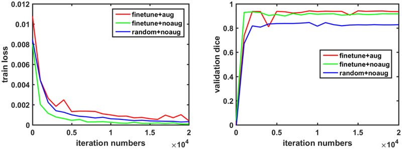
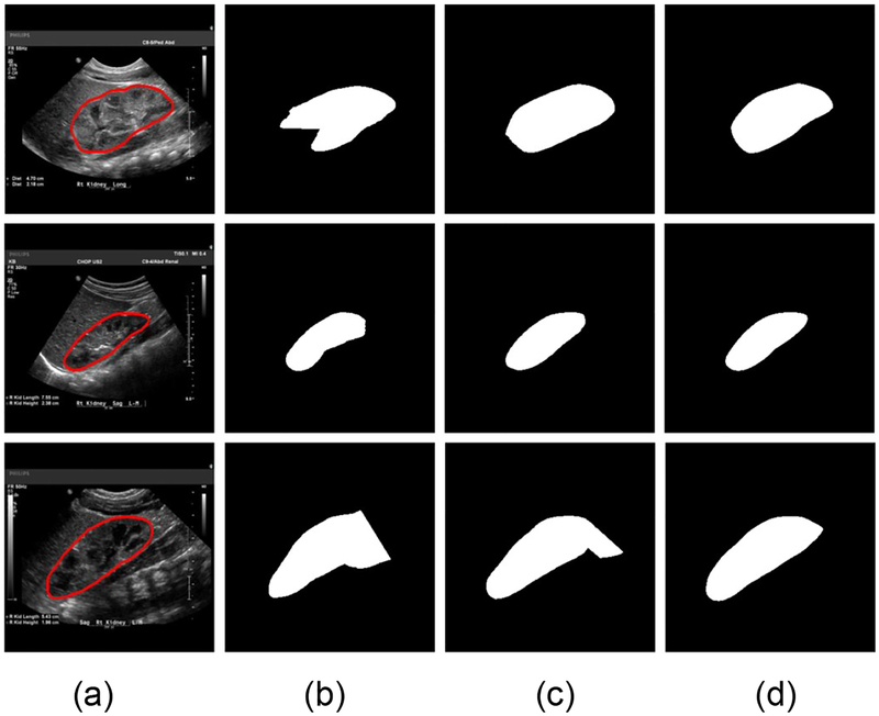
Fig. 10 shows traces of the training loss and validation accuracy of the kidney boundary detection network trained with 3 different training strategies. These traces demonstrate that the training of the kidney boundary distance regression network converged regardless of the training strategies used. Without the data augmentation, the transfer-learning strategy made the model to better fit the training data and obtained better segmentation accuracy than the random initialization strategy. Although the train loss was relatively larger if the network was trained based on the augmented data, better validation segmentation accuracy was obtained. Validation segmentation accuracy measures of different training strategies are summarized in Table 2 and example segmentation results are illustrated in Fig. 11, further demonstrating that the transfer learning and data augmentation strategies could make the boundary detection network to achieve better results. The results were obtained at 9000, 1000, 16000 iteration numbers respectively with the different training strategies according to their validation accuracy traces.

Fig. 10.

Traces of the training loss (left) and validation accuracy (right) associated with 3 different training strategies.

Table 2.

Segmentation performance of different training strategies on the validation dataset.

Methods	random+noaug	finetune+noaug	finetune+aug
Dice	0.8458±0.1714	0.9338±0.0377	0.9421±0.0343
MD	6.1173±4.7427	3.2896±2.0465	3.0804±2.7781

Fig. 11.

Example segmentation results obtained with 3 training strategies. (a) input image and ground truth boundary, (b) results of the training from scratch without data augmentation, (c) results of the transfer learning without data augmentation, and (d) results of the transfer-learning with data augmentation.

3.2. Performance of the kidney boundary detection networks trained using different lambda settings

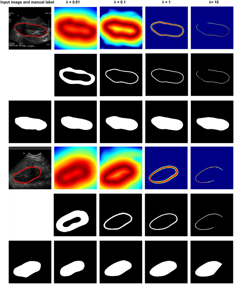
Fig. 12 shows example kidney boundaries and masks obtained by the boundary detection networks trained with different distance maps in the validation dataset. Particularly, the kidney masks were closer to the ground truth when the distance maps were normalized with λ = 1 than other values. When λ= 0.01, the detected boundaries were much wider than the ground truth, while when λ = 10 or λ = 0.1, the detected boundaries missed some pixels. Such a problem could be overcome to some extent by the post-processing steps, including morphological operations and minimum spanning tree. As summarized in Table 3, the kidney segmentation results obtained with λ = 0.1 and λ = 1 were comparable, better than those obtained with other parameters. It is worth noting that predicted boundary distance regression results shown in Fig. 12 were not binary maps when λ = 1 or 10. We set λ = 1 in all following experiments. We also found that the softmax cross-entropy loss function based pixelwise classification network classified all the pixels into background due to the unbalanced samples.

Fig. 12.

Results of the kidney boundary detection networks trained using different loss functions. The 1^st and 4^rd rows show predicted boundary distance maps, the 2^st and 5^rd rows show boundary binary maps, and the 3^nd and 6^th rows show kidney masks obtained by the morphology operation and minimum spanning tree based post-processing method.

Table 3.

Segmentation results of the boundary detection network trained with distance functions with different settings on the validation dataset.

	λ = 0.01	λ = 0.1	λ = 1	λ = 10
Dice	0.9003±0.0978	0.9364±0.0501	0.9421±0.0343	0.9264±0.0593
MD	4.2726±3.4268	2.8683±1.9569	3.0804±2.7781	3.3180±2.7279

3.3. Segmentation performance of the kidney boundary detection and pixel classification networks

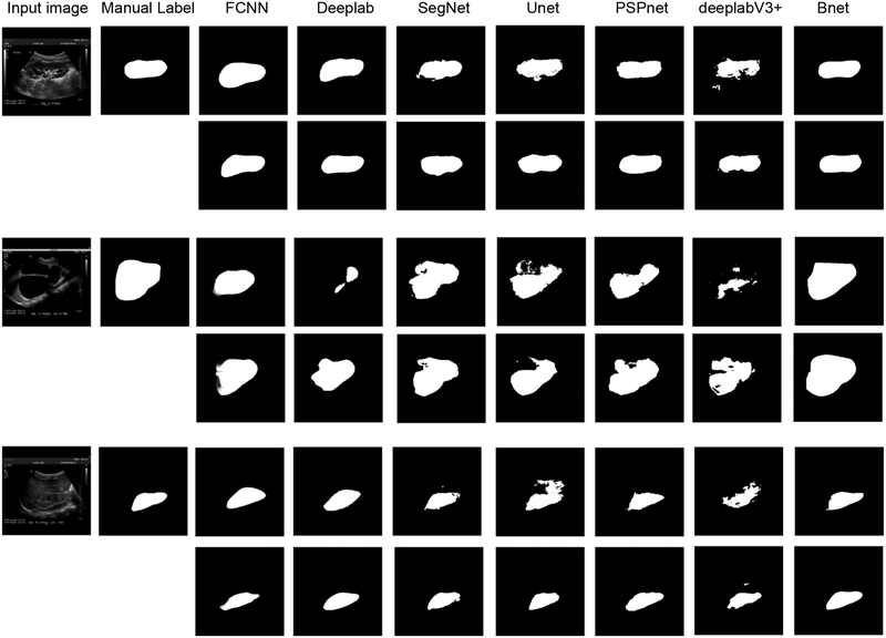
Table 4 and Table 5 show kidney segmentation results of the testing data obtained by FCNN, Deeplab, SegNet, Unet, PSPnet, deeplabV3+, and the boundary detection network (Bnet), trained without the data augmentation or with the data augmentation. The morphology operation and minimum spanning tree based post-processing method was used to obtain kidney masks from the boundary detection network. The results demonstrate that the boundary detection networks had significantly better performance than the alternative deep learning segmentation networks that were trained to classify pixels into kidney and non-kidney pixels. The results also demonstrated that the data-augmentation could improve the performance of all the methods under comparison. Fig. 13 shows representative segmentation results obtained by the deep learning methods under comparison with or without the data augmentation. These results demonstrate that our method had robust performance regardless of the variance of kidney shape and appearance. However, the alternative methods under comparison had relatively worse performance.

Table 4.

Comparison results for the proposed method and other methods without data augmentation on the testing dataset.

	Dice coefficient		Mean distance		Jaccard		Sensitivity		Precision		ASSD
	Mean±std	p-value	Mean± std	p-value	Mean± std	p-value	Mean±std	p-value	Mean± std	p-value	Mean±std	p-value
FCNN	0.8020±0.1037	3.1e–27	9.6083±4.8746	4.1e–26	0.6806±0.1316	1.4e–27	0.7614±0.1404	1.1e–25	0.8690±0.1118	1.7e–15	9.9992±5.4128	1.2e–27
Deeplab	0.8724±0.0639	8.4e–26	6.2596±2.9087	2.0e–21	0.7788±0.0899	7.1e–26	0.8759±0.1002	3.2e–12	0.8829±0.0788	2.9e–19	6.3022±3.1650	8.8e–25
SegNet	0.8894±0.0619	2.9e–20	7.3921±6.1747	2.2e–23	0.8061± 0.0949	1.6e–20	0.8809±0.0917	5.4e–9	0.9080±0.0814	2.3e–10	6.1979±4.6609	4.8e–21
Unet	0.8899±0.0578	1.7e–20	7.5227±4.1757	8.8e–26	0.8062±0.0883	1.2e–20	0.8780±0.0900	4.7e–12	0.9121±0.0745	5.8e–09	6.2147±3.3764	7.9e–24
PSPnet	0.8869±0.0548	2.0e–22	7.2514±4.0461	3.2e–23	0.8008±0.0828	1.0e–22	0.8818±0.0885	6.1e–10	0.9027±0.0741	4.4e–16	6.0621±3.0109	4.7e–22
Deeplabv3+	0.8965±0.0698	2.4e–13	6.4669±3.8065	1.9e–18	0.8187±0.1014	2.0e–13	0.8643±0.1100	9.6e–13	0.9424±0.0474	-	5.3100±2.9109	5.7e–16
Bnet	0.9303±0.0499	-	3.6130±2.3447	-	0.8729±0.0708	-	0.9220±0.0690	-	0.9442±0.0482	-	3.4792±1.9618	-

Table 5.

Comparison results for the proposed method and other methods with data augmentation on the testing dataset.

	Dice coefficient		Mean distance		Jaccard		Sensitivity		Precision		ASSD
	Mean±std	p-value	Mean± std	p-value	Mean± std	p-value	Mean±std	p-value	Mean± Std	p-value	Mean±std	p-value
FCNN	0.9179±0.0471	4.8e–17	4.2072±2.4922	4.2e–16	0.8514±0.0731	2.4e–17	0.9221±0.0730	4.8e–06	0.9207±0.0622	6.0e–10	4.1182±2.3157	1.5e–16
Deeplab	0.9236±0.0370	1.9e–18	3.7369±1.8737	4.5e–14	0.8601±0.0603	1.3e–18	0.9175±0.0584	3.0e–15	0.9344±0.0528	1.9e–03	3.7779±1.8596	1.6e–16
SegNet	0.9298±0.0409	2.3e–11	4.0753±6.4316	3.6e–10	0.8713±0.0651	1.6e–11	0.9311±0.0542	2.1e–05	0.9330±0.0600	2.0e–04	3.8450±4.9187	8.9e–10
Unet	0.9245±0.0403	2.7e–14	4.0987±2.5463	5.8e–14	0.8620±0.0650	2.6e–14	0.9132±0.0621	3.3e–13	0.9423±0.0614	4.3e–02	3.8643±2.1498	1.1e–14
PSPnet	0.9372±0.0305	1.8e–05	3.3055±2.0240	2.7e–04	0.8837±0.0580	3.4e–04	0.9491±0.0440	-	0.9292±0.0577	1.0e–09	3.1471 ± 1.6704	1.7e–03
DeeplabV3+	0.9311±0.0354	2.8e–08	3.5080±2.2860	5.0e–05	0.8732±0.0610	1.7e–05	0.9307±0.0517	1.6e–05	0.9369±0.0612	2.1e–03	3.1837±1.9855	8.1e–05
Bnet	0.9427±0.0453	-	2.9189±1.9823	-	0.8943±0.0663		0.9439±0.0645		0.9458±0.0413	-	2.8701±1.8671

Fig. 13.

Representative segmentation results obtained by different deep learning networks trained without data augmentation (the 1^st, 3^nd, and 5^rd rows) and with data augmentation (the 2^th, 4^th, and 6^th rows).

Table 6 summarizes 5-fold cross-validation results obtained by the proposed subsequent segmentation networks, PSPnet and Deeplab. These results indicated that our method obtained significantly better performance than alternative deep learning methods on the most evaluation metrics, except Sensitivity.

Table 6.

Five-fold cross-validation results obtained by the subsequent segmentation, PSPnet, and Deeplab.

		PSPnet	Deeplab	Proposed
Dice coefficient	Mean±std	0.9255±0.0839	0.9155±0.0921	0.9304±0.0703
	p-value	3.9e–3	7.3e–10
Mean distance	Mean±std	3.7955±4.6565	4.8282±5.1308	3.0977±2.8955
	p-value	4.9e–5	7.2e–21
Jaccard	Mean±std	0.8699±0.1110	0.8543±0.1223	0.8763±0.0992
	p-value	4.3e–3	6.2e–10
Sensitivity	Mean±std	0.9454±0.0416	0.9461±0.0682	0.9301±0.0739
	p-value	2.8e–4	1.5e–15
Precision	Mean±std	0.9187±0.1175	0.8970±0.1213	0.9378±0.0832
	p-value	1.4e–9	1.7e–36
ASSD	Mean±std	3.5030±3.6718	4.1403±3.8713	3.0338±2.4152
	p-value	2.3e–3	1.0e–14

3.4. Comparison of the subsequent segmentation networks, the boundary detection network, and the multi-task learning based segmentation network

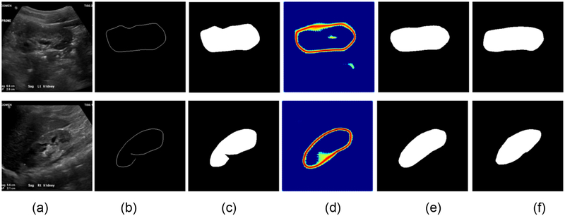
Table 7 shows segmentation performance of the kidney boundary detection network and the subsequent boundary distance regression and pixelwise classification networks, demonstrating that the end-to-end learning could obtain better performance, although the difference was not statistically significant (p>0.05). Fig. 14 indicated that the proposed framework could improve the boundary detection segmentation results with blurring boundaries. More importantly, we could obtain kidney masks from their distance maps without any post-processing step. As illustrated by intermediate results shown in Fig. 14(d), the end-to-end networks obtained distance maps as expected. A further comparison of computational time costs of two solutions indicated that the end-to-end learning was 20 times faster than the morphology and minimum spanning tree based post-processing.

Table 7.

Comparison results for the proposed model with only distance loss function and end-to-end subsequent segmentation framework on the testing dataset.

	Boundary detection network	End-to-end learning
Dice	0.9427±0.0453	0.9451±0.0315
MD	2.9189±1.9823	2.6822±1.4634
Time (sec)	3.75	0.18

Fig. 14.

Results for the boundary detection network and the end-to-end learning networks. (a) input kidney US images, (b) binary skeleton maps of the predicted distance maps, (c) kidney masks obtained with the minimum spanning tree based post-processing, (d) predicted distance maps obtained by the end-to-end subsequent segmentation networks, (e) kidney masks obtained by the end-to-end subsequent segmentation network, and (f) kidney masks obtained by manual labels.

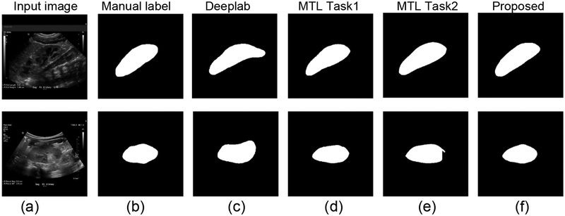
Table 8 summarizes segmentation accuracy measures obtained by the multi-task learning and the subsequent segmentation networks. Fig. 15 shows segmentation results of two representative kidney images, obtained by the multi-task learning and the subsequent segmentation networks. Particularly, the multi-task learning network’s individual tasks had different performance. Particularly, the pixelwise classification network (task 1) had worse performance than the boundary detection network (task 2), and all of them had significantly worse performance than the subsequent segmentation network. Interestingly, the multi-task network-task1 had better performance than the Deeplab segmentation network (Table 5).

Table 8.

Comparison results for the subsequent segmentation network and the multi-task learning network on the testing dataset.

	Dice		MD
	Mean±std	p-value	Mean±std	p-value
Subsequent networks	0.9451±0.0315	-	2.6822±1.4634	-
Multi-task network-task1 (classification)	0.9119±0.0569	1.1e–20	4.4555±2.4292	7.8e–24
Multi-task network-task2 (regression)	0.9314±0.0345	4.6e–12	3.3148±1.6704	1.7e–12

Fig 15.

Results for the multi-task learning based segmentation network and the end-to-end learning networks. (a) input kidney US images, (b) manual label, (c) results obtained by Deeplab, (d) results obtained by task 1 of the multi-task learning (MTL) network, (e) results obtained by task 2 of the MTL network, and (f) results obtained by the subsequent segmentation network.

3.5. Segmentation performance of our method on rotated testing kidney images and testing kidney images with boundary cut

Table 9 summarizes segmentation performance of the subsequent segmentation network on the rotated testing kidney images. The results indicated that our segmentation model was relatively robust to the kidney orientation when absolute value of the rotation degree was relatively small, although it obtained the best performance on the testing images without rotation (Dice index = 0.9451±0.0315).

Table 9.

Dice index values of segmentation results of the testing images rotated by different degrees.

Rotation (degree)	−5	−10	−15	−30
Dice index (mean±std)	0.9433±0.0330	0.9431±0.0320	0.9426±0.0339	0.9393±0.0401
Rotation (degree)	5	10	15	30
Dice index (mean±std)	0.9438±0.0272	0.9421±0.0290	0.9388±0.0325	0.9231±0.0505

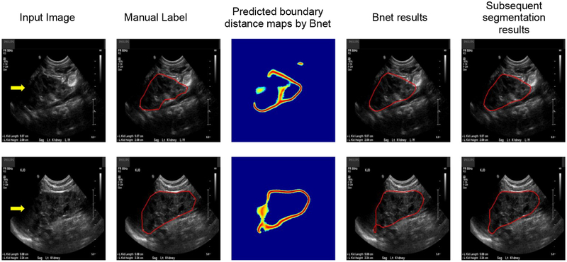
As illustrated by Fig. 16, the boundary detection network obtained degraded boundary distance maps for images with boundary cut. The proposed post-processing method could obtain a good segmentation result for the image shown on the top row, but did not work well for the one shown on the bottom row. However, the subsequent segmentation network obtained better segmentation results for both the images. Table 10 summarizes segmentation performance obtained by the boundary detection network and the subsequent segmentation network on the 21 testing kidney images with the boundary cut, indicating that the subsequent segmentation network performed significantly better on the kidney images with the boundary cut.

Fig 16.

Example segmentation results of kidney images with boundary cut. The boundary cut is indicated by the yellow arrows.

Table 10.

Comparison results for the Bnet and end-to-end subsequent segmentation networks on the kidney images with boundary cut

	Dice		MD
	Mean±std	p-value	Mean±std	p-value
Boundary detection network	0.8201±0.1788	2.3e–02	8.0299±5.5013	3.3e–02
Subsequent segmentation network	0.8529±0.1463	-	6.1673±5.7510	-

4. DISCUSSION

In this study, we propose a novel boundary distance regression network architecture to achieve fully-automatic kidney segmentation. The boundary distance regression network is integrated with a subsequent pixelwise classification network to achieve improved kidney segmentation performance in an end-to-end learning fashion, instead of directly learning a pixelwise classification neural network to distinguish kidney pixels from non-kidney ones. Our method has been evaluated for segmenting clinical kidney US images with large variability in both appearance and shape, yielding significantly better performance than the alternatives under comparison. Our results have demonstrated that the boundary detection strategy worked better than pixelwise classification techniques for segmenting clinical US images although the pixelwise classification techniques have demonstrated excellent image segmentation performance in a variety of image segmentation problems, including FCNN (Long et al., 2015), Deeplab (Chen et al., 2018b), SegNet (Badrinarayanan et al., 2017), Unet (Ronneberger et al., 2015), PSPnet (Zhao et al., 2017), and DeeplabV3+(Chen et al., 2018a). Our results have also demonstrated that the kidney shape registration-based data-augmentation method could improve the segmentation performance.

Compared with kidney US image segmentation methods built upon level-set techniques that require either manual operations or image registration to initialize the level-set functions (Marsousi et al., 2017; Zheng et al., 2018b), the proposed subsequent segmentation network method directly works on the input kidney images without any intermediate processing steps, an important aspect that would increase uptake in clinical medicine. Our method obtained segmentation results with similar accuracy as the semi-automatic kidney US image segmentation method (Zheng et al., 2018b), but at a much higher speed, which again increases its clinical utility. Our method is built upon the kidney boundary detection. However, the kidney boundaries in US images could be corrupted by shady or blurry artifacts, which could affect the image segmentation accuracy, as illustrated by Fig. 16. For the kidney images with boundary cut, the subsequent segmentation network obtained significantly better performance than the boundary detection network. The method could also be improved by adopting statistical shape modeling techniques that have demonstrated promising performance for segmenting 3D kidney US images (Marsousi et al., 2017). Our method has been only evaluated based on the kidney images in sagittal view. In the present study, the images in sagittal view images were chosen manually and a fully automatic method is needed to automate this process.

Though our kidney segmentation network is built on the pre-trained VGG16 network, our model is not limited to the VGG network. Within the same framework, we could also adopt other semantic segmentation networks with good performance in natural images segmentation tasks, such as ResNet (He et al., 2016) or networks built on VGG19 (Simonyan and Zisserman, 2014), which may further improve the performance of the kidney segmentation results. Moreover, our method could be further improved by incorporating multi-scale learning strategies that have demonstrated helpful in image segmentation (Chen et al., 2018a; Zhao et al., 2017).

5. CONCLUSIONS

We have developed a fully automatic method to segment kidneys in clinical ultrasound images by integrating boundary distance regression and pixel classification networks subsequently in an end-to-end learning framework. Experimental results have demonstrated that the boundary distance regression network could robustly detect boundaries of kidneys with varied shapes and heterogeneous appearances in clinical ultrasound images, and the end-to-end learning of subsequent boundary distance regression and pixel classification networks could effectively improve the performance of automatic kidney segmentation, significantly better than deep learning-based pixel classification networks.

Fig. 9.

A multi-task learning based segmentation networks (top) under comparison with the proposed subsequent segmentation network. In both the networks, the boundary detection (boundary distance regression) network and the pixelwise classification network shared the same transfer learning network.

REFERENCES

- Ardon R, Cuingnet R, Bacchuwar K, Auvray V, 2015. Fast kidney detection and segmentation with learned kernel convolution and model deformation in 3D ultrasound images, 2015 IEEE 12th International Symposium on Biomedical Imaging (ISBI), pp. 268–271. [Google Scholar]
- Badrinarayanan V, Kendall A, Cipolla R, 2017. SegNet: a deep convolutional encoder-decoder architecture for image segmentation. IEEE Transactions on Pattern Analysis and Machine Intelligence 39, 2481–2495. [DOI] [PubMed] [Google Scholar]
- Bertasius G, Shi J, Torresani L, 2015. High-for-low and low-for-high: Efficient boundary detection from deep object features and its applications to high-level vision, Proceedings of the IEEE International Conference on Computer Vision, pp. 504–512. [Google Scholar]
- Bookstein FL, 1989. Principal warps: thin-plate splines and the decomposition of deformations. IEEE transactions on pattern analysis and machine intelligence 11, 567–585. [Google Scholar]
- Boyd S, Vandenberghe L, 2004. Convex optimization. Cambridge university press. [Google Scholar]
- Cerrolaza JJ, Safdar N, Biggs E, Jago J, Peters CA, Linguraru MG, 2016. Renal segmentation from 3D ultrasound via fuzzy appearance models and patient-specific alpha shapes. IEEE Transactions on Medical Imaging 35, 2393–2402. [DOI] [PubMed] [Google Scholar]
- Cerrolaza JJ, Safdar N, Peters CA, Myers E, Jago J, Linguraru MG, 2014. Segmentation of kidney in 3D-ultrasound images using Gabor-based appearance models, 2014 IEEE 11th International Symposium on Biomedical Imaging (ISBI), pp. 633–636. [Google Scholar]
- Chen H, Qi X, Yu L, Dou Q, Qin J, Heng P-A, 2017. DCAN: deep contour-aware networks for object instance segmentation from histology images. Medical Image Analysis 36, 135–146. [DOI] [PubMed] [Google Scholar]
- Chen L-C, Barron JT, Papandreou G, Murphy K, Yuille AL, 2016. Semantic image segmentation with task-specific edge detection using cnns and a discriminatively trained domain transform, Proceedings of the IEEE Conference on Computer Vision and Pattern Recognition, pp. 4545–4554. [Google Scholar]
- Chen L-C, Zhu Y, Papandreou G, Schroff F, Adam H, 2018a. Encoder-decoder with atrous separable convolution for semantic image segmentation. Springer International Publishing, Cham, pp. 833–851. [Google Scholar]
- Chen L, Papandreou G, Kokkinos I, Murphy K, Yuille AL, 2018b. DeepLab: semantic image segmentation with deep convolutional nets, atrous convolution, and fully connected CRFs. IEEE Transactions on Pattern Analysis and Machine Intelligence 40, 834–848. [DOI] [PubMed] [Google Scholar]
- Glorot X, Bengio Y, 2010. Understanding the difficulty of training deep feedforward neural networks, Proceedings of the thirteenth international conference on artificial intelligence and statistics, pp. 249–256. [Google Scholar]
- Hao Y, Wang T, Zhang X, Duan Y, Yu C, Jiang T, Fan Y, Alzheimer’s Disease Neuroimaging I, 2014. Local label learning (LLL) for subcortical structure segmentation: application to hippocampus segmentation. Human brain mapping 35, 2674–2697. [DOI] [PMC free article] [PubMed] [Google Scholar]
- He K, Zhang X, Ren S, Sun J, 2016. Deep residual learning for image recognition, The IEEE Conference on Computer Vision and Pattern Recognition, pp. 770–778. [Google Scholar]
- Jackson P, Hardcastle N, Dawe N, Kron T, Hofman MS, Hicks RJ, 2018. Deep learning renal segmentation for Fully automated radiation Dose estimation in Unsealed source Therapy. Frontiers in oncology 8. [DOI] [PMC free article] [PubMed] [Google Scholar]
- Jun X, Yifeng J, Hung-tat T, 2005. Segmentation of kidney from ultrasound images based on texture and shape priors. IEEE Transactions on Medical Imaging 24, 45–57. [DOI] [PubMed] [Google Scholar]
- Kruskal JB, 1956. On the shortest spanning subtree of a graph and the traveling salesman problem. Proceedings of the American Mathematical society 7, 48–50. [Google Scholar]
- Li C, Wang X, Liu W, Latecki LJ, Wang B, Huang J, 2019a. Weakly supervised mitosis detection in breast histopathology images using concentric loss. Medical Image Analysis 53, 165–178. [DOI] [PubMed] [Google Scholar]
- Li H, Jiang G, Zhang J, Wang R, Wang Z, Zheng W-S, Menze B, 2018. Fully convolutional network ensembles for white matter hyperintensities segmentation in MR images. NeuroImage 183, 650–665. [DOI] [PubMed] [Google Scholar]
- Li Y, Liu H, Li H, Fan Y, 2019b. Feature-Fused Context-Encoding Network for Neuroanatomy Segmentation. arXiv:1905.02686. [DOI] [PMC free article] [PubMed]
- Long J, Shelhamer E, Darrell T, 2015. Fully convolutional networks for semantic segmentation, Proceedings of the IEEE conference on computer vision and pattern recognition, pp. 3431–3440. [DOI] [PubMed] [Google Scholar]
- Marsousi M, Plataniotis KN, Stergiopoulos S, 2017. An Automated Approach for Kidney Segmentation in Three-Dimensional Ultrasound Images. IEEE J Biomed Health Inform 21, 1079–1094. [DOI] [PubMed] [Google Scholar]
- Martí;n-Fernández M, Alberola-López C, 2005. An approach for contour detection of human kidneys from ultrasound images using Markov random fields and active contours. Medical Image Analysis 9, 1–23. [DOI] [PubMed] [Google Scholar]
- Men K, Geng H, Zhong H, Fan Y, Lin A, Xiao Y, A deep learning model for predicting xerostomia due to radiotherapy for head-and-neck squamous cell carcinoma in the RTOG 0522 clinical trial. International Journal of Radiation Oncology • Biology • Physics. [DOI] [PMC free article] [PubMed] [Google Scholar]
- Mendoza CS, Kang X, Safdar N, Myers E, Martin AD, Grisan E, Peters CA, Linguraru MG, 2013. Automatic analysis of pediatric renal ultrasound using shape, anatomical and image acquisition priors, In: Mori K, Sakuma I, Sato Y, Barillot C, Navab N (Eds.), Medical Image Computing and Computer-Assisted Intervention – MICCAI 2013. Springer Berlin Heidelberg, Berlin, Heidelberg, pp. 259–266. [DOI] [PubMed] [Google Scholar]
- Meola M, Samoni S, Petrucci I, 2016. Imaging in chronic kidney disease. Contributions to nephrology 188, 69–80. [DOI] [PubMed] [Google Scholar]
- Noble JA, Boukerroui D, 2006. Ultrasound image segmentation: a survey. IEEE Transactions on medical imaging 25, 987–1010. [DOI] [PubMed] [Google Scholar]
- Ozmen CA, Akin D, Bilek SU, Bayrak AH, Senturk S, Nazaroglu H, 2010. Ultrasound as a diagnostic tool to differentiate acute from chronic renal failure. Clin Nephrol 74, 46–52. [PubMed] [Google Scholar]
- Pulido JE, Furth SL, Zderic SA, Canning DA, Tasian GE, 2014. Renal parenchymal area and risk of ESRD in boys with posterior urethral valves. Clinical journal of the American Society of Nephrology : CJASN 9, 499–505. [DOI] [PMC free article] [PubMed] [Google Scholar]
- Ravishankar H, Venkataramani R, Thiruvenkadam S, Sudhakar P, Vaidya V, 2017. Learning and incorporating shape models for semantic segmentation, International Conference on Medical Image Computing and Computer-Assisted Intervention Springer, pp. 203–211. [Google Scholar]
- Ronneberger O, Fischer P, Brox T, 2015. U-net: Convolutional networks for biomedical image segmentation, International Conference on Medical image computing and computer-assisted intervention Springer, pp. 234–241. [Google Scholar]
- Sharma K, Peter L, Rupprecht C, Caroli A, Wang L, Remuzzi A, Baust M, Navab N, 2015. Semi-automatic segmentation of autosomal dominant polycystic kidneys using random forests. arXiv preprint arXiv:1510.06915. [DOI] [PMC free article] [PubMed]
- Sharma K, Rupprecht C, Caroli A, Aparicio MC, Remuzzi A, Baust M, Navab N, 2017. Automatic segmentation of kidneys using deep learning for total kidney volume quantification in autosomal dominant polycystic kidney disease. Scientific reports 7, 2049. [DOI] [PMC free article] [PubMed] [Google Scholar]
- Simonyan K, Zisserman A, 2014. Very deep convolutional networks for large-scale image recognition. arXiv preprint arXiv:1409.1556.
- Tang H, Moradi M, Wong KC, Wang H, El Harouni A, Syeda-Mahmood T, 2018. Integrating deformable modeling with 3D deep neural network segmentation, Deep Learning in Medical Image Analysis and Multimodal Learning for Clinical Decision Support. Springer, pp. 377–384. [Google Scholar]
- Torres HR, Queirós S, Morais P, Oliveira B, Fonseca JC, Vilaça JL, 2018. Kidney segmentation in ultrasound, magnetic resonance and computed tomography images: A systematic review. Computer Methods and Programs in Biomedicine 157, 49–67. [DOI] [PubMed] [Google Scholar]
- Woolson RF, 2008. Wilcoxon signed-rank test. Wiley Encyclopedia of Clinical Trials, 1–3. [Google Scholar]
- Xie S, Tu Z, 2015. Holistically-nested edge detection, The IEEE International Conference on Computer Vision, pp. 1395–1403. [Google Scholar]
- Yin S, Zhang Z, Li H, Peng Q, You X, Furth S, Tasian G, Fan Y, 2019. Fully-automatic segmentation of kidneys in clinical ultrasound images using a boundary distance regression network. Proceedings of 2019 IEEE International Symposium on Biomedical Imaging (ISBI), 1–4. [DOI] [PMC free article] [PubMed] [Google Scholar]
- Zhao H, Shi J, Qi X, Wang X, Jia J, 2017. Pyramid scene parsing network, Proceedings of the IEEE conference on computer vision and pattern recognition, pp. 2881–2890. [Google Scholar]
- Zhao X, Wu Y, Song G, Li Z, Fan Y, Zhang Y, 2016. Brain Tumor Segmentation Using a Fully Convolutional Neural Network with Conditional Random Fields, In: Crimi A, Menze B, Maier O, Reyes M, Winzeck S, Handels H (Eds.), Brainlesion: Glioma, Multiple Sclerosis, Stroke and Traumatic Brain Injuries. Springer International Publishing, Cham, pp. 75–87. [Google Scholar]
- Zhao X, Wu Y, Song G, Li Z, Zhang Y, Fan Y, 2018a. 3D Brain Tumor Segmentation Through Integrating Multiple 2D FCNNs, In: Crimi A, Bakas S, Kuijf H, Menze B, Reyes M (Eds.), Brainlesion: Glioma, Multiple Sclerosis, Stroke and Traumatic Brain Injuries. Springer International Publishing, Cham, pp. 191–203. [Google Scholar]
- Zhao X, Wu Y, Song G, Li Z, Zhang Y, Fan Y, 2018b. A deep learning model integrating FCNNs and CRFs for brain tumor segmentation. Medical image analysis 43, 98–111. [DOI] [PMC free article] [PubMed] [Google Scholar]
- Zheng Q, Furth SL, Tasian GE, Fan Y, 2019. Computer aided diagnosis of congenital abnormalities of the kidney and urinary tract in children based on ultrasound imaging data by integrating texture image features and deep transfer learning image features. Journal of Pediatric Urology 15, 75.e71–75.e77. [DOI] [PMC free article] [PubMed] [Google Scholar]
- Zheng Q, Tasian G, Fan Y, 2018a. Transfer learning for diagnosis of congenital abnormalities of the kidney and urinary tract in children based on ultrasound imaging data, 2018 IEEE 15th International Symposium on Biomedical Imaging (ISBI 2018), pp. 1487–1490. [DOI] [PMC free article] [PubMed] [Google Scholar]
- Zheng Q, Warner S, Tasian G, Fan Y, 2018b. A dynamic graph cuts method with integrated multiple feature maps for segmenting kidneys in 2D ultrasound images. Academic Radiology 25, 1136–1145. [DOI] [PMC free article] [PubMed] [Google Scholar]
- Zheng Q, Wu Y, Fan Y, 2018c. Integrating semi-supervised and supervised learning methods for label fusion in multi-atlas based image segmentation. Frontiers in Neuroinformatics 12, 69. [DOI] [PMC free article] [PubMed] [Google Scholar]