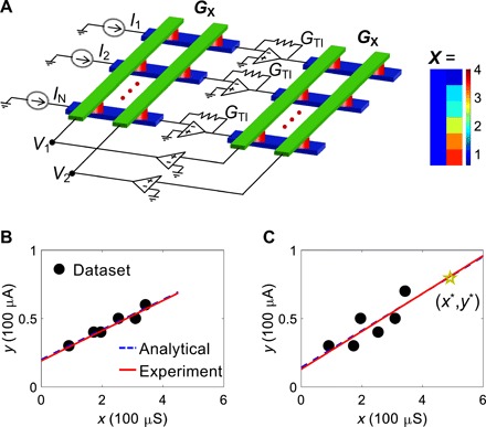
Fig. 1. Linear regression circuit and experiments.

(A) Schematic illustration of the cross-point circuit for solving linear regression with the pseudoinverse method. The conductance transformation unit is G₀ = 100 μS. The feedback conductance G_TI of TIA is equal to G₀. A representative matrix X for simple linear regression of six data points is also shown. (B) Linear regression of a six-point dataset defined by the second column of X in (A) on the x axis and the input currents on the y axis. The figure also shows the analytical and experimental regression lines, and the latter being obtained as the measured voltages v in the cross-point circuit as regression weights. (C) A second six-point regression experiment with the same vector X in (A) and a different set of input currents. A new input value x* = 4.91 was stored in an additional line of the left cross-point array, thus enabling the one-step prediction along a sequence. The measured prediction y* = 0.727 is consistent with experimental and analytical regression lines.