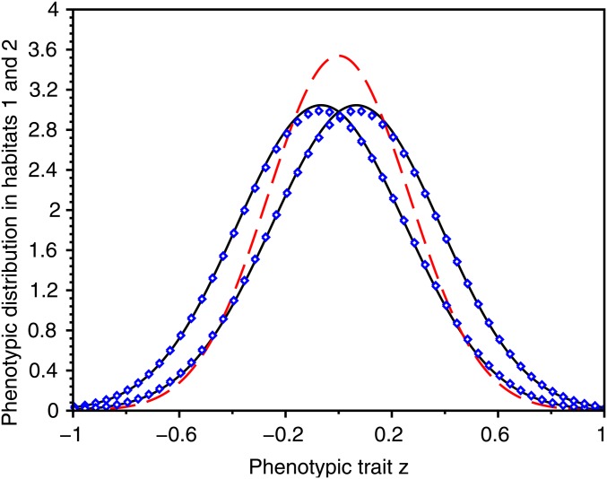
Figure 3.

Selection–mutation–migration equilibrium of the phenotypic densities $n_{\epsilon ,i}\left(z\right)$ in the two habitats in a symmetric scenario. We plot the exact phenotypic densities at equilibrium obtained from numerical computations of the equilibrium of Equation 3 (blue dots) together with our first approximation (full black line) in a case where the distribution is unimodal in each habitat. We also plot the approximation given in Débarre et al. (2013) (red dashed line). Note that our approximation captures the emergence of some differentiation, even though we are above the critical migration rate leading to the evolution of a dimorphic population. In the presence of large mutation rates, the population distribution is indeed shifted to the left (respectively right) in the first (respectively second) habitat, while Débarre et al. (2013) provided the same approximation for both habitats. Our calculation yields also better approximations for the variance of the distribution in each habitat (Débarre et al. 2013 underestimates this variance). In this and the following figures, to compute the equilibrium numerically, we have solved the dynamic problem numerically (Equation 3) and kept the solution obtained for a long time after equilibrium has been reached. Parameter values: $m=1.5$, $r_{\text{max}}=3$, $s=2$; $\theta =0.5$, $\kappa =1$, $U=1$, $\epsilon =0.1$.