Figure 3.

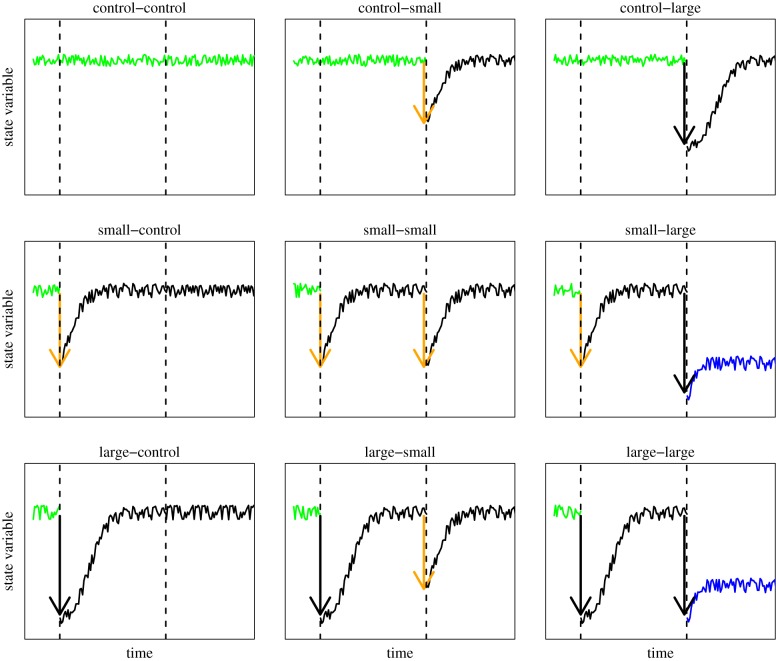
A theoretical example of the nine possible treatment combinations of a manipulative experiment that applies multiple perturbations (two in this case) of different amplitude and monitors the response of state variables (e.g. biomass) over time. The green line represents natural fluctuations before any perturbation as in the control–control scenario (top left corner). Perturbations (arrows) can be applied at one of two points in time (vertical horizontal lines) and with small (orange arrow) or large (black arrow) amplitude. Here, we assume that the state variable drops after being perturbed and then starts to recover. Depending on the sequence and amplitude of perturbations, the state variable may recover to its original state or settle onto a new state (blue solid line). Here, we assume that a late and large perturbation makes the system shift to a new alternative stable state (see small–large and large–large scenarios) while one large perturbation in isolation does not necessarily shift the system to a new stable state. This is a specific assumption to illustrate just one of the possible outcomes. We also assume that the new state has an equilibrium at a lower level than the original one. The full experimental design would consist of nine treatments (all possible alternations of control, small and large) and multiple spatial replicates for each combination of treatments. The temporal resolution of measurements (frequency of data collection and time between the two pulses) will depend on the nature of the state variable and its natural temporal variability. Perturbations can also be of a different nature (e.g. drought versus flood), which combined with the size of the perturbation would further increase the complexity of the experimental design.