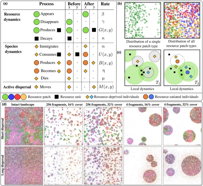
Figure 1.

(a). Overview of the model. Rows represent processes which turn entities in positions x and y (‘before’ column) into a new configuration (‘after’ column) at given rates (last column). The Greek letters are positive constants, G and U are top‐hat kernels, and B and M are Gaussian kernels (see SI text for details). (b) Illustration of the large‐scale environmental variation in habitat types. The panels show a snapshot of the sinusoidal resource patch distributions in an intact 100 × 100 continuous landscape. (c) Example cartoon of local dynamics over time in a continuous 4 × 4 area contained in a larger landscape. T ₁: Resource‐deprived individuals immigrate into the area. They consume resources that are within their utilisation radius (gray area). T ₂: some individuals have become resource‐satiated by consuming resource units, and have produced offspring into their surroundings within distance δ (dotted circles). (d) Snapshots of simulations with eight species in landscapes with varying degree of fragmentation and habitat cover in a continuous 100 × 100 landscape. The top row shows a scenario with δ = 1 and bottom row a scenario with δ = 10, both with passive dispersal. Coloured dots represent species individuals (larger ones are resource‐satiated and smaller are resource‐deprived individuals, respectively). The resource patches, resource units and habitat fragments are not drawn. In both cases the matrix is habitable.