A spatially explicit empirical model of structural development processes in natural forests based on climate and topography

Abstract

Stand structure develops with stand age. Old‐growth forests with well‐developed stand structure support many species. However, development rates of stand structure likely vary with climate and topography. We modeled structural development of 4 key stand variables and a composite old‐growth index as functions of climatic and topographic covariates. We used a hierarchical Bayesian method for analysis of extensive snap‐shot National Forest Inventory (NFI) data in Japan (n = 9244) to account for differences in stand age. Development rates of structural variables and the old‐growth index exhibited curvilinear responses to environmental covariates. Flat sites were characterized by high rates of structural development. Approximately 150 years were generally required to attain high values (approximately 0.8) of the old‐growth index. However, the predicted age to achieve specific values varied depending on environmental conditions. Spatial predictions highlighted regional variation in potential structural development rates. For example, sometimes there were differences of >100 years among sites, even in the same catchment, in attainment of a medium index value (0.5) after timber harvesting. The NFI data suggested that natural forests, especially old natural forests (>150 years), remain generally on unproductive ridges, steep slopes, or areas with low temperature and deep snow, where many structural variables show slow development rates. We suggest that maintenance and restoration of old natural forests on flat sites should be prioritized for conservation due to the likely rapid development of stand structure, although remaining natural forests on low‐productivity sites are still important and should be protected.

Short abstract

Article impact statement: Forest structural development rates vary depending on the environment, and in Japan plantations occupy areas where rates of development of stand structure are fast.

Introduction

Forests regrow after harvesting at different rates due to the heterogeneous distribution of environmental conditions that influence site productivity (Perry et al. 2008). These include local factors, such as fine‐scale topography (slope position, slope angle, aspect, etc.), soil type, water and nutrient availability, windiness (Curt et al. 2001), and regional‐ to continental‐climatic conditions, such as temperature, precipitation, and snow cover (McKenney & Pedlar 2003). Environmental controls of forest growth are particularly important because environments are globally changing rapidly (Kirilenko & Sedjo 2007).

Stand structure is the horizontal and vertical distribution of forest components, including tree height and diameter, depth and extent of the crown, and presence and abundance of snags and down woody debris (Helms 1998). Stand structure changes with forest growth and typically becomes more complex over time, a process referred to as stand structural development (Franklin et al. 2002). Old‐growth forests are characterized by horizontally and vertically diverse structural attributes (Spies 1997; Franklin et al. 2002) and have many environmental values, such as biodiversity conservation, carbon sequestration, and hydrological regulation (Barlow et al. 2016; Lutz et al. 2018; Watson et al. 2018).

Because old‐growth forests are becoming increasingly scarce worldwide (Mackey et al. 2015; Potapov et al. 2017), indicators of structural complexity have been developed to help identify stands with high conservation value (McElhinny et al. 2005; van Galen et al. 2018). One of these indicators is an old‐growth index, which was devised to distinguish old‐growth Douglas fir (Pseudotsuga menziesii) stands in western North America based on 4 key structural variables of a stand: mean tree diameter at breast height (dbh), density of large Douglas fir trees (>100 cm dbh), standard deviation (SD) of tree dbh, and tree density (Acker et al. 1998; Zenner 2004; Whitman & Hagan 2007). In old‐growth forests, the first 3 and the fourth variables typically have large and small values, respectively. An advantage of the old‐growth index is its use of common stand variables that can be calculated readily from tree plot data. These structural variables are also likely to distinguish temperate old‐growth forests in other parts of the world (Burrascano et al. 2013).

Close relationships between forest growth and structural development suggest that site productivity influences development rates of forest structure following disturbance (Franklin et al. 2002). Using the old‐growth index, Larson et al. (2008) demonstrated that, after timber harvesting, forest structure develops most rapidly on productive sites. This suggests that there may be substantial spatial heterogeneity in structural development rates. However, because Larson et al. (2008) used measured tree heights as a proxy of site productivity, it remains unclear which and how environmental factors drive spatial heterogeneity in structural development rates.

Local drivers of site productivity (e.g., topography, soil types, soil nutrients, wetness, and local climate) have been measured in intensive field surveys (e.g., Curt et al. 2001). However, topography can be represented by a digital elevation model (DEM). Other local drivers, which are affected by topography (Swanson et al. 1988), can also be represented by a DEM (Moore et al. 1993). For example, topography influences soil formation (Perry et al. 2008) and can be used to predict tree biomass as an alternative of soil properties (de Castilho et al. 2006). Furthermore, regional to continental climates can be incorporated into the models of site productivity (McKenney & Pedlar 2003; Nothdurft et al. 2012). Therefore, it is possible to model structural development based on spatially explicit environmental covariates.

Our objective was to model structural development processes in natural forests based on climate and topography with the extensive plot data from Japan's National Forest Inventory (NFI) (n = 9244 plots). We tested a series of hypotheses (Table 1) to answer the following question: What are the relationships between the development rates of structural variables and climatic and topographic covariates? We used hierarchical Bayesian modeling (Gelman & Hill 2007; Royle & Dorazio 2008), which enabled us to infer underlying structural development processes based on snap‐shot NFI data and to account for differences in stand age among plots (Fig. 1 & Supporting Information). We then applied the model to predict potential structural development rates and values for the old‐growth index across a 20 × 20 km region in central Japan. Maintaining and restoring old‐growth forests may be a key conservation goal (Watson et al. 2018), and we sought to further this objective.

Table 1.

Possible effects of 6 climatic and topographic covariates on development rates of forest structure

Covariate	Possible effect (reason)a	This studyb	Reference
Climate
snow depth	negative (as snow depth increases, growth period shortens) unimodal (many tree species have a common optimal climate under which sampled environmental conditions vary widely)	mean dbh: unimodal tree density: positive* large tree density: positive SD of dbh: positive* old‐growth index: positive*	Peterson & Peterson 2001 Nothdurft et al. 2012
warmth index	positive (as the temperature increases, the growth period increases) unimodal (many tree species have a common optimal climate when the sampled environmental conditions vary widely)	mean dbh: negative tree density: negative large tree density: unimodal SD of dbh: unimodal old‐growth index: negative*	McKenney & Pedlar 2003 Nothdurft et al. 2012
Topography
slope angle	negative (steep slope induces soil movement and tree fall)	mean dbh: negative* tree density: negative* large tree density: positive SD of dbh: neutral old‐growth index: negative	Guariguata 1990
terrain openness (positive openness)	unimodal (concave terrain [small terrain openness] induces soil movement and tree fall; convex terrain [high terrain openness] induces water and nutrient deficiencies; flat terrain has a rapid forest growth rate due to high soil moisture and nutrients)	mean dbh: unimodal tree density: negative large tree density: positive SD of dbh: neutral old‐growth index: neutral	Hunter & Parker 1993; Chen et al. 1998; Curt et al. 2001
catchment area	positive (lower part of slope has rapid forest growth rate due to high soil moisture and nutrients)	mean dbh: positive* tree density: positive* large tree density: positive* SD of dbh: positive* old‐growth index: positive*	Chen et al. 1998; Curt et al. 2001
solar radiation	negative (greater solar radiation induces water deficiency in the temperate zone)	mean dbh: negative* tree density: negative* large‐tree density: positive SD of dbh: negative* old‐growth index: negative*	Chen et al. 1998; Fekedulegn et al. 2003; Mitsuda et al. 2007

^aPossible effects and mechanisms are from studies on forest and tree growth (or site productivity).

^bBased on the significance of parameter estimates at 5% level. When both simple and quadratic terms were significant (*, indicating nonlinear or curvilinear decrease or increase), the effects of simple terms had higher priority for simplicity. Abbreviation: dbh, diameter breast height.

Figure 1.

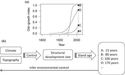
Structural development processes and modeling scheme. (a) Four hypothetical trajectories (A–D) of forest structural development processes that initiated in different years (black circles, states of stand structure surveyed by National Forest Inventory); different forest plots had different stand age (also shown in [b]) and different rates of structural development, which could yield different stand structure even with similar stand age. (b) Structural development rates driven by climate and topography and stand structure driven by stand age and development rates (also shown in [a]). We inferred these latent (unobserved) environmental controls and structural development processes given stand structure, stand age, climate, and topography by assuming they followed the series of formulations in Eqs. 2 and 3.

Methods

Plot Data and Usage

Japan's NFI forest monitoring system consists of >13,000 permanent plots on a 4‐km, country‐wide lattice grid. The survey commenced in 1999 and required 5 years to complete a survey of all plots. We obtained stand variables from the plots of natural forests (i.e., we excluded plantations comprising 35% of the data from the analysis). We used all available plot data collected from 1999 to 2013 (4729 plots in which 1934 and 2581 plots were measured 3 and 2 times, respectively) (see Supporting Information for the treatment of NFI data). Tree species composition of Japan's natural forests is influenced by a thermal gradient, specifically a warmth index (corresponding to the period of plant growth) calculated by summing monthly mean temperatures >5°C (Kira 1991). We used only those NFI data within 45–180 for the warmth index to focus on the deciduous and evergreen broad‐leaved forests (cool‐ and warm‐temperate forests [Kira 1991]), which are 2 major forest types in Japan. We excluded subarctic and subtropical forests.

Based on the successful application of an old‐growth index in the United States (e.g., Acker et al. 1998; Zenner 2004; Whitman & Hagan 2007) and the relationships between structural variables and stand age (derived from forest registers) in our NFI data, we used the following 4 structural variables to distinguish Japanese old‐growth forests from younger stands: mean dbh of live trees with >5 cm dbh, density of live trees with 40 cm dbh (large tree density/ha), SD of dbh for live trees with >5 cm dbh, and density of live trees with >5 cm dbh (Supporting Information). The first 3 and the fourth variables typically increase and decrease with stand age, respectively. The correlation coefficients between the 4 structural variables were |0.31|–|0.73| (Supporting Information).

Climate and Topography Covariates

We used maximum snow depth and the warmth index as climate covariates in our model, both of which are known to affect tree species composition across Japan (Kira 1991; Nakashizuka & Iida 1995), possibly because of their effects on tree survival and regeneration processes (Supporting Information). We used Climate Mesh Data 2000 published by Japan's Meteorological Agency (1‐km resolution) to generate values for these 2 covariates (Supporting Information). We obtained data on topographical covariates (slope angle, terrain [positive] openness, catchment area [surrogate for soil moisture and nutrients] (Table 1), and solar radiation [Supporting Information]), which are known to influence forest growth and structure (e.g., Guariguata 1990; Mitsuda et al. 2007), from a 20‐m DEM based on a 10‐m DEM published by the Geospatial Information Authority of Japan (Supporting Information). We used ArcGIS 10.3 Spatial Analyst extension (ESRI, Redlands, California, U.S.A.) and SAGA GIS (Conrad et al. 2015) for geospatial analyses.

Model Structure

Following the earlier definition of the old‐growth index, we formulated the old‐growth index (I _og) to have values from 0 to 1:

$$I_{\mathrm{og}}=\mathrm{mean}\left(I_{i,\mathrm{og}}\right)=\frac{1}{4}\times \sum _{i=1}^4\left|\frac{x_i-x_{i,\mathrm{young}}}{x_{i,\mathrm{old}}-x_{i,\mathrm{young}}}\right|,$$ (1)

where x_i is the ith structural variable, x_{i, young} is the median value of x_i for young forests derived from the plot data, and x_{i, old} is the median value of x_i for qualified old‐growth forests in Japan. This formulation means I _og is a mean value of 4 subindices calculated from 4 structural variables (I_{i ,og}). We used median values rather than mean values, as employed by Acker et al. (1998), to reduce the effects of outliers. Although Larson et al. (2008) obtained x_{i ,young} from 40‐ to 80‐year‐old forests, the stand ages of interest in this study included forests <40 years old because Japan is dominated by young forests (Yamaura et al. 2012). We then set x_{i ,young} by using the plot data from ≤10‐ to 30‐year‐old forests (Supporting Information). To obtain x_{i, old}, we used median values from 18 permanent plots registered as old‐growth deciduous and evergreen broad‐leaved forests (>150 years old) in Japan (Ishihara et al. 2010). This simplification enabled us to analyze the national data set with a single criterion (median value) for each structural variable. We did not find clear differences in structural variables between deciduous and evergreen broad‐leaved forests except for live tree density (Supporting Information). Live tree density also varied little between young and old growth forests; however, we incorporated this variable into the analysis because its development rates showed a dependency on topographic covariates. Nevertheless, modeled environmental dependency for the rates of development of old‐growth index remained mainly unchanged when live tree density was excluded (Supporting Information). We assigned x_{i, young} or x_{i, old} for the values of x_i beyond the range of x_{i, young} and x_{i, old}, and delimited I_{i ,og} within 0 and 1. Although live tree density decreases with stand age, older stands can have higher indices due to the use of absolute values in Eq. 1.

We then examined the effects of environmental covariates on development rates of I _og and the 4 subindices (I_{i ,og}). Following Larson et al. (2008) and Warton and Hui (2011), we logit transformed these proportional data (I _og and I_{i, og}) and regressed stand age (explanatory variables) on logit‐transformed proportions (as response variables):

$$\begin{array}{ccc}& & \log \left(I_{\mathrm{og},j}/\left[1-I_{\mathrm{og},j}\right]\right)={\beta }_0+\mathrm{coef}{\mathrm{f}}_j\times \mathrm{ag}{\mathrm{e}}_j\hfill \\ & & +\mathrm{plot}.\mathrm{ef}{\mathrm{f}}_{\mathrm{site}\left[j\right]}+\mathrm{period}.\mathrm{ef}{\mathrm{f}}_{\mathrm{term}\left[j\right]}+e_j,\hfill \end{array}$$ (2)

where I _{og, j} is the old‐growth index of the jth sample (plot data), age_j is its stand age, β ₀ is an intercept, coeff_j is a coefficient of stand age (can be specific to the jth sample) that dictates structural development rates (Larson et al. 2008), plot.eff is a random plot effect because the same plots could be measured multiple times, and period.eff is a fixed‐effect term that captures the possible effects of measurement period by first and second periods relative to the latest third period (third period was treated as a reference category). As the initial phase of model development for the old‐growth index, we made the intercept constant across the plots to simplify the model following Larson et al. (2008) (but see Supporting Information). Subscripts site (j) and term (j) denote the identity of the plots and measurement periods for jth sample. The final term (e_j) is an unexplained error term with a normal distribution. A challenge in this method is the inability to deal with possible maximum and minimum proportional values (1 and 0) because the denominator of the logit transformation cannot take a value of 0 (I _og = 1) and its logarithm cannot take 0 (I _og = 0). We therefore added to, or subtracted from, the minimum nonzero values, called ε (Supporting Information), the possible minimum or maximum values (0 or 1 values in proportion) that allowed the application of logit‐transformed regression (Warton & Hui 2011).

We examined effects of environmental covariates on structural development rates by modeling coeff_j as the function of covariates:

$$\mathrm{coef}{\mathrm{f}}_j={\beta }_1+\sum _k\left({\beta }_{k,1}{x}_{k,j}+{\beta }_{k,2}{x}_{k,j}^2\right),$$ (3)

where β ₁ is an intercept, x_k,j is the kth covariate of the jth site, and β_{k ,1} and β_{k ,2} are coefficients of x_k,j and its squared term, respectively. Using a quadratic model, we considered the possible nonlinear effects of covariates. Although we also constructed low‐rank thin‐plate splines (one of the generalized linear models) that can deal with more complex functional forms, modeled effects were mostly blurred and not significant (Supporting Information). We therefore used this relatively simple quadratic model (cubic models also yielded the similar results with quadratic models). Our model was hierarchical in that the slope for stand age (coeff_j) in Eq. 2 was a function of covariates in Eq. 3 (varying‐slope model [Gelman & Hill 2007]).

Our approach allowed the use of snap‐shot plot data from stands of different age (Fig. 1). Specifically, each stand can have different structural development rates (coeff_j), depending on the values of environmental covariates (Eq. 3), and their development after disturbance follows logistic curves (Eq. 2). Current development (I _og) is therefore the product of these processes with specific period (stand age). In other words, given current stand and environmental data and the assumed model formulations, we inferred the latent underlying development processes and their possible environmental dependencies (parameters of Eqs. 2 & 3).

Because our NFI data set had 2 consecutive pairs of the structural variables at the same plots, we compared the 4 variables between third and second periods and second and first periods. It was shown that more recent data sets had generally larger values (Supporting Information), which was inconsistent with the expected pattern for live tree density (typically decreases with stand age). This may be due to underestimated tree densities in the older periods of field surveys (Forestry Agency 2017b ). We therefore incorporated the effects of measurement period in Eq. 2 (period.eff). As an independent data set, we also examined the longitudinal permanent plot data from Ishihara et al. (2010). We derived structural variables from 7 plots of broad‐leaved forests <100 years old with 5–13 years of longitudinal surveys (mean [SD] = 9.9 years [2.5]). The temporal changes of structural variables generally exhibited the expected pattern (Supporting Information). Although we did not include these permanent data in our analysis, their inclusion did not change the obtained results due to their small sample size. In our model, although we simplified variable trajectories of structural development processes depending on a range of factors, such as disturbance history (Spies 1997), we could flexibly alter the model structure. For example, we could consider variability in initial conditions in the intercept of Eq. 2, decadal climatic variability in Eq. 3, or both.

Model Fitting

To estimate relationships between covariates and structural development rates, we fitted the models (Eqs. 2 & 3) for the old‐growth index (I _og) and for 4 subindices (I_{i, og}). We standardized each covariate to enhance convergence (Kéry & Royle 2016) and stabilized estimates, especially quadratic terms (Schielzeth 2010). Although there was limited correlation between most covariates (|r| <0.3), snow depth and warmth index (−0.57) and positive openness and catchment area (−0.62) were highly correlated (Supporting Information). Highly correlated covariates are not always detrimental to an analysis and can be required to explain variations in response variables (e.g., Hamilton 1987). We therefore fitted these correlated covariates simultaneously because we considered that they likely had different ecological meanings and our sample size was large. We also confirmed that parameter estimates remained qualitatively unchanged when we excluded one of the pairs of covariates from the model.

We estimated parameters with Markov Chain Monte Carlo analysis with JAGS version 4.2.0 (Plummer 2013), jagsUI version 1.3.7 (Kellner 2015), and R version 3.2.3 (R Core Team 2015) software. We used conventional vague priors, ran 3 chains with different initial values, discarded the initial 100 iterations, and ran an additional 10,000 iterations to examine the posterior distributions (change of the prior distributions did not affect the estimates [Supporting Information]). Chain convergence was achieved when the $\overline{R}$ statistic was <1.1 for parameter estimates; otherwise, an additional 10,000 iterations were conducted until convergence in the autojags function in jagsUI. We calculated the coefficient of determination (R ²) from the Pearson correlation coefficient between observed and predicted values at logit scale. To calculate R ², we excluded random plot effects but included measurement period effects in Eq. 2. We also tested the model performance by cross‐validation (holdout method). We randomly chose 90% of the data for model training and tested the model with the 10% of remaining data. We repeated this procedure 100 times and obtained R ² at each repetition. We did not undertake model selection because many covariates had significant effects (their 95% CI did not include zero) such that we could compare the fitted functional forms among the structural variables given the large sample size (Supporting Information).

Mapping Indices

To demonstrate the utility of our models, we made spatial predictions of the old‐growth index for natural forests in northern Ibaraki Prefecture, central Japan (between the cities of Kitaibaraki and Takahagi). We compiled relevant climate, topographic, and stand (forest type and stand age) covariates based on the above‐described methods for every 20‐m resolution grid. We derived stand covariates from forest registers.

Because our model for the old‐growth index treated structural development processes and stand age as functions of climate and topography, we could estimate the stand age required to attain a certain value of the old‐growth index under specific environmental conditions. Following Larson et al. (2008), we inferred these ages at values of 0.5 old‐growth index (t _0.5) for every 20‐m grid.

We constructed the model of the old‐growth index substituting parameter estimates (posterior means) and environmental covariates for each grid and equated the linear predictor (right‐hand side of Eq. 2 without random plot and measurement period effects) with 0 (meaning 0.5 value of the index). We then numerically solved this equation for stand age (i.e., obtained corresponding stand age [t _0.5]) with the uniroot function in R. To prevent model extrapolation, we replaced the environmental covariates beyond 95% of the data used for model construction by 97.5% or 2.5% quantile values in predictions.

We also produced a map of predicted values (given the current stand age) of old‐growth index for natural forests. Mean and median posterior estimates were almost the same, and t _0.5 predicted by mean and median estimates was also almost the same and was highly correlated (r > 0.99). Finally, we compared the environmental covariates among old natural forests (>150 years old), other natural forests, and major plantation forests in NFI data. We only used the latest third‐period data and did not screen plots by the warmth index.

Results

Modeling Structural Development Processes

Our 4 structural variables, as well as the old‐growth index, exhibited varied and curvilinear responses in their development rates to 6 climatic and topographic covariates (Fig. 2). Mean dbh and tree density were the most sensitive and SD of dbh showed similar response, but its environmental dependency was not as strong. The density of large trees was also not sensitive but showed unique responses, and the old‐growth index had an intermediate response to the 4 structural variables. Specifically, tree density showed clear positive responses to snow depth. Tree density and mean dbh exhibited negative responses to the warmth index. Responses of mean dbh to snow depth and large‐tree density and SD of dbh to the warmth index were unimodal. Structural variables (except for large‐tree density) had consistent negative responses to slope angle and solar radiation, and large‐tree density showed only positive responses to these covariates. Structural variables exhibited varied responses to terrain openness. All structural variables consistently showed positive responses to catchment area.

Figure 2.

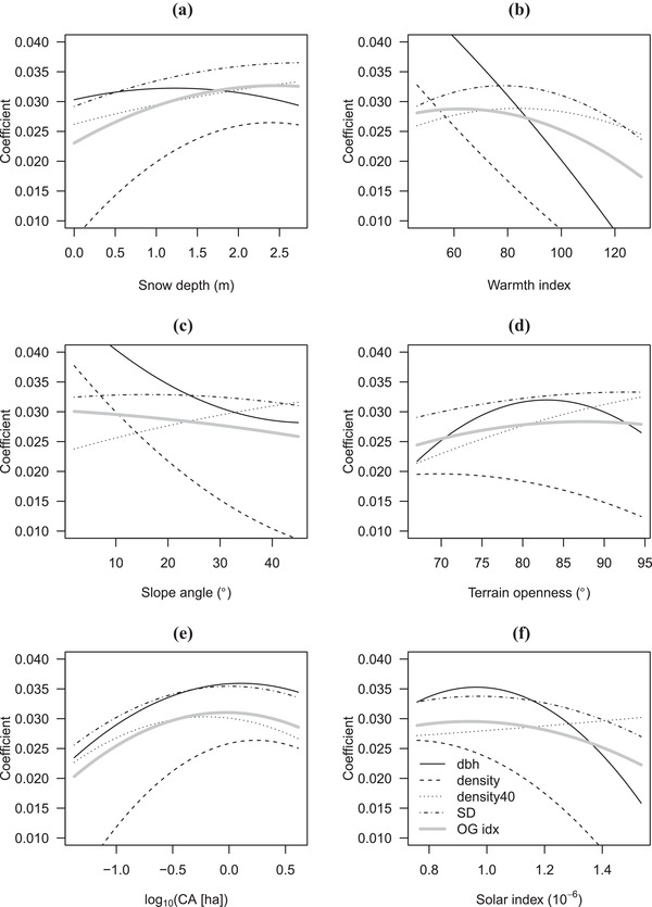
Modeled dependency of 4 forest structural variables and old‐growth index on 6 environmental covariates (dbh, mean diameter at breast height for live trees; density, density of live trees; density 40, density of live trees with 40 cm dbh; SD, standard deviation of dbh for live trees; OG idx, old‐growth index; CA, catchment area). Fitted lines are derived from Eq. 3 and shown in the range of 95% percentiles of environmental covariates. Other covariates were held constant at mean values. See Supporting Information for their corresponding 95% CIs.

Inferred logistic curves showed large unexplained variation in measured structural variables and the old‐growth index (Fig. 3 & Supporting Information). The R ² ranged from 0.23 (mean dbh) to 0.31 (SD of dbh), and cross validation yielded 0.02‐0.03 SD of R ² around these values (Supporting Information). For example, many plots approximately 50 years old (most common stand age) had higher values for the old‐growth index than predicted by the model (Fig. 3 & Supporting Information). Our results suggested that 150 years was generally required for natural forests to attain high values (approximately 0.8) for the old‐growth index; the specific age to achieve such values varied depending on plot‐level environmental conditions. Snow depth, warmth index, catchment area, and solar radiation had large effects on the forms of logistic curves (Fig. 3). We also found significant measurement‐period effects. While accounting for stand‐age differences given the model structure, the first and second periods of plot measurements produced smaller values of 4 structural variables and old‐growth index compared with the third period (Supporting Information). These deviations were generally larger in the older first period than in the second period.

Figure 3.

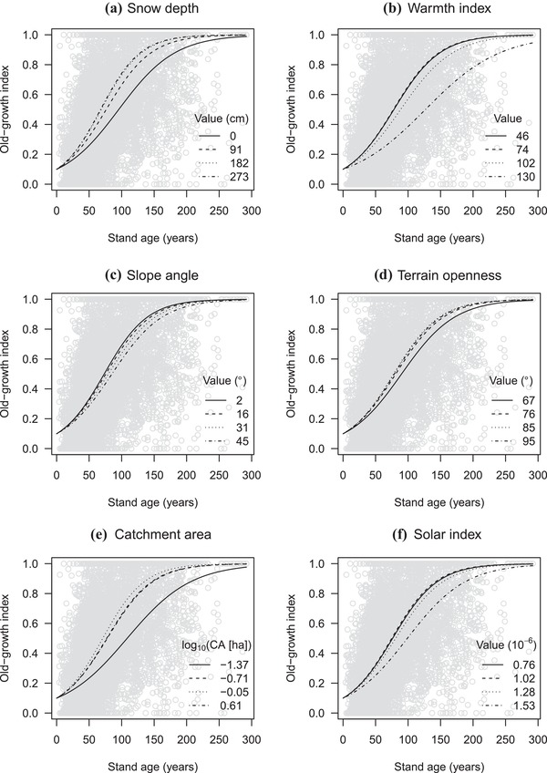
(a–f) Inferred logistic curves of old‐growth index relative to stand age for 6 environmental covariates (CA, catchment area). Curves with different covariate values (within the 95% percentiles) are depicted. For example, (b) shows 4 fitted lines with 4 different values of warmth index (0.025 and 0.975 quantiles and their intermediate values). Other covariates were held constant at mean values. Effects of measurement period are not included (assuming they are from the third period).

Model Prediction

Predicted stand age to achieve a 0.5 value for the old‐growth index (t _0.5) showed spatial heterogeneity in structural development rates associated with climate and topography (Figs. 4c & 4d). Eastern grids had higher t _0.5 (low development rates) due to higher temperatures and limited snow (Fig. 4c). In each catchment, flat valley bottoms had low t _0.5, whereas ridges and steep slopes had high t _0.5 (Figs. 4c & 4d). Large values of t _0.5 were spatially clustered in some areas due to complex terrain (Fig. 4c & Supporting Information). Predicted values of the old‐growth index exhibited substantial spatial heterogeneity (Fig. 4b), and high values were found in the west, where old natural forests occur (Fig. 4b & Supporting Information).

Figure 4.

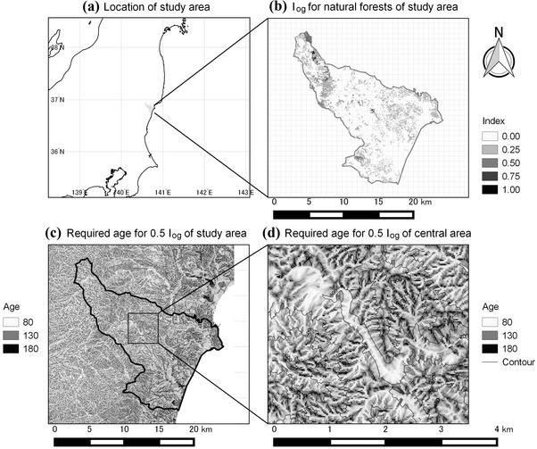
Spatial prediction of structural development processes based on the series of parameter estimates (Eqs. 2 & 3) and associated environmental covariates: (a) location of study area, (b) predicted old‐growth index (I _og) for natural forests in the study area, (c) predicted stand age required to achieve a 0.5 I _og (t _0.5) in northern Ibaraki prefecture, and (d) predicted stand age required to achieve a 0.5 I _og (t _0.5) incenter of study area. Estimates of I _og are available only for natural forests within the middle of the study area (b), where forest‐register data are available. See Supporting Information for the spatial distribution of environmental covariates.

Environmental Condition Among Forest Types

The NFI data showed that site conditions differed between natural and plantation forests in Japan. Environments supporting natural forests, especially those for old forests, were typically in the areas with deep snow, low temperatures, and large slope angle (Fig. 5). Japanese cedar and cypress plantations, which are 2 primary species of plantations in Japan, have been established in the warmer parts of Japan; cedar plantations dominated the areas with large catchment areas at which development rates of natural forests are high. Japanese red pine plantations were an exception; they have been established in locations with small catchment area.

Figure 5.

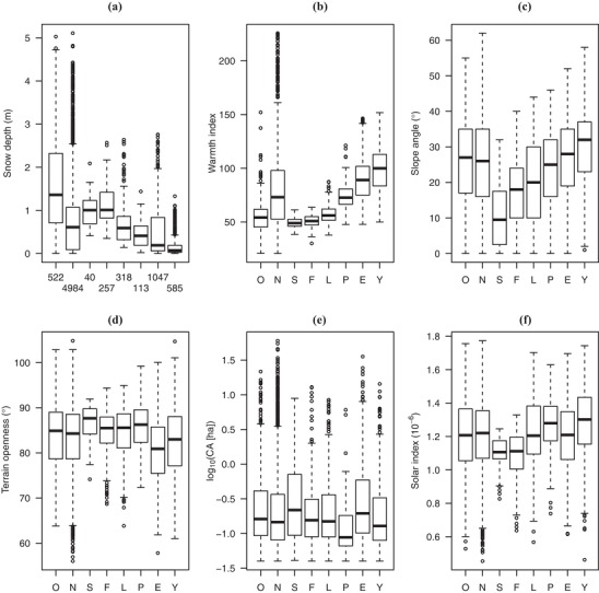
(a–f) Relationship between 6 environmental covariates and 8 forest types covered by National Forest Inventory data (O, natural forest >150 years old; N, natural forest ≤150 years old; S, Sakhalin spruce [Picea glehnii] plantation; F, Sakhalin fir [Abies sachalinensis] plantation; L, Japanese larch [Larix kaempferi] plantation; P, Japanese red pine [Pinus densiflora] plantation; E, Japanese cedar plantation; Y, Japanese cypress [Chamaecyparis obtuse] plantation; CA, catchment area; boxes, 25th and 75th percentiles [interquartile range]; whiskers, minimum and maximum values within 1.5 times interquartile range from interquartile range; horizontal line within bars, median; circles, outliers). In (a), numbers along the horizontal axis indicate the number of plots for the respective forest types shown on the x‐axes of the other graphs.

Discussion

To the best of our knowledge, we are the first to spatially evaluate structural development processes of natural forests at a regional scale. Our results suggest that old natural forests remain on unproductive areas, where many structural variables have slow rates of development. Our findings also highlighted the conservation importance of old natural forests on flat areas. Given the current scarcity of old‐growth forests and the heterogeneous distribution of rates of structural development, our empirical modeling is useful for assessing the impacts of current land use from the perspective of biodiversity conservation.

Structural Development Processes and Environment

Mean and SD of dbh and large‐tree density showed unimodal responses to snow depth and the warmth index. Unimodal responses are consistent with the growth rates of a range of tree species in relation to precipitation and temperature from southwest Germany (Nothdurft et al. 2012). There may be common optimal climate conditions for these structural variables. Low structural development rates in areas characterized by deep snow and low temperatures are most likely explained by a short growth period (Peterson & Peterson 2001). Clear positive and negative responses by tree density to snow depth and warmth index, respectively, were partially because evergreen broad‐leaved old‐growth forests in southwestern Japan had high tree densities (Supporting Information).

However, low structural development rates for other variables in areas with limited snow and higher temperatures may not be explained by declines in growth rates but rather by long‐term and intensive forest use by humans. Evergreen broad‐leaved forests have 2 times larger annual net primary production as deciduous broad‐leaved forests, which dominate northeastern Japan (Kira 1991). Japan's southern forests, where warm temperatures and limited snow allow people to use forests throughout the year, have been exploited heavily (Totman 1989). This is consistent with the evidence of there being few old, natural forests (Fig. 5) and natural forests (Yamaura et al. 2011) in those areas in Japan.

Sites with steep slopes or concave terrain were likely to have low development rates for many structural variables. This is most likely due to high soil movement and elevated rates of tree fall (Guariguata 1990). It is also well known that sites with small catchment areas and exposed (convex) topography, such as ridges, have impaired forest growth rates (Curt et al. 2001). An unexpected result was that large‐tree density increased with slope angle and terrain openness. The inaccessibility of steep sites and ridges may lead to reduced human disturbance and in turn more large old trees (Pederson 2010). Solar radiation intensity had mostly negative effects, which was consistent with studies on forest growth rates (Chen et al. 1998) and suggests that water deficiency can also affect structural development rates.

Old‐Growth Index as an Indicator of Forest Biodiversity

Forest structure is a well‐known indicator of forest biodiversity (Lindenmayer et al. 2000), and the old‐growth index may be a potentially useful composite indicator. Identifying forests with developed structure and high conservation value was a key motivation for devising the old‐growth index (Spies & Franklin 1988, 1991; Whitman & Hagan 2007). Because our model treated the index as a function of stand age, it is straightforward to forecast the future status of old growth in landscapes subject to different kinds of forest management. The old‐growth index comprises common stand variables, and our environmental covariates were also derived from a DEM and a GIS. Our framework is therefore broadly applicable to other regions.

Our results showed that fine‐grained (20‐m resolution) topographic factors can lead to differences in structural development rates (Figs. 4c & 4d). This scale intersects well with the scale of forest management ownership and decision making. For example, 74% of Japanese forest owners have holdings of 1–5 ha (Forestry Agency 2017c ). In our mapping area, the mean [SD] size of the stand area of natural forests was 0.73 [2.38] ha. It has been suggested that fine‐scale topography provides the underlying setting for ecosystem processes and human land uses (Swanson et al. 1988). It was predicted that topographic features throughout a landscape could lead to differences in >100 years to attain an old‐growth index of 0.5 after harvesting, even within the same catchment (Fig. 4d). We suggest the consideration of topography would be useful for the spatial evaluation of biodiversity and ecosystem services and would go beyond, for example, land use and cover as simple proxies for them (Rieb et al. 2017).

Temporal Changes in Measurement Error

Our results showed that older surveys that have measured structural variables could yield smaller values. Surveyors can miss trees at the margins of circular plots or measure dbh of tree trunks at a height taller than the prescribed height, which is especially likely for complex‐shaped broad‐leaved trees (Forestry Agency 2017a ). Underestimation of the SD can be the products of these 2 processes. Accuracy of measurement has been improving since surveyors completed field training from 2011 (Forestry Agency 2017a , 2017b ). Therefore, there is a risk of overestimating development rates without considering these measurement errors.

Limitations and Implications

Although we simplified our model to allow for scaling up and did not analyze tree species composition and coarse woody debris, these compositional and structural forest attributes characterize different forest development stages and have important functions, such as habitat provision (e.g., Franklin et al. 2002). Relatively large amounts of variation remained unexplained by our model, indicating the potential for model improvement (e.g., with other local information, such as disturbance history and soil type; incorporating environmental covariates into the intercept; and direct modeling of annual changes in structural variables from repeated surveys) (Supporting Information).

Our results suggest that the replacement of natural forests by plantation forests is not a spatially random process. Natural forests, especially old natural forests, remain generally on unproductive ridges, steep slopes, or areas with severe climatic conditions (Fig. 5), where many key attributes of stand structure develop slowly (Fig. 2). Therefore, the impacts of replacement of natural forests by plantations are larger than those indicated by the spatial extent of converted areas alone. The maintenance and restoration of old‐growth forest on flat sites should be prioritized for conservation, although natural forests on unproductive sites will continue to be important and should be protected.

Supporting information

Descriptions about NFI data (Appendix S1), treatment of structural variables and model structure (Appendix S2), graphical plots of structural variables and varied models (Appendix S3), environmental covariates (Appendix S4), graphical plots of model outputs (Appendix S5), results of cross‐validation (Appendix S6), environmental covariates for spatial prediction (Appendix S7), modeling issue of Eq. 2 (Appendix S8), parameter estimates (Appendix S9), and source R codes of the analysis (Appendix S10) are available online. The authors are solely responsible for the content and functionality of these materials. Queries (other than absence of the material) should be directed to the corresponding author.

Literature Cited

- Acker SA, Sabin TE, Ganio LM, McKee WA. 1998. Development of old‐growth structure and timber volume growth trends in maturing Douglas‐fir stands. Forest Ecology and Management 104:265–280. [Google Scholar]
- Barlow J, et al. 2016. Anthropogenic disturbance in tropical forests can double biodiversity loss from deforestation. Nature 535:144–147. [DOI] [PubMed] [Google Scholar]
- Burrascano S, Keeton WS, Sabatini FM, Blasi C. 2013. Commonality and variability in the structural attributes of moist temperate old‐growth forests: a global review. Forest Ecology and Management 291:458–479. [Google Scholar]
- Chen HYH, Klinka K, Kabzems RD. 1998. Site index, site quality, and foliar nutrients of trembling aspen: relationships and predictions. Canadian Journal of Forest Research 28:1743–1755. [Google Scholar]
- Conrad O, Bechtel B, Bock M, Dietrich H, Fischer E, Gerlitz L, Wehberg J, Wichmann V, Böhner J. 2015. System for Automated Geoscientific Analyses (SAGA) v. 2.1.4. Geoscientific Model Development 8:1991–2007. [Google Scholar]
- Curt T, Bouchaud M, Agrech G. 2001. Predicting site index of Douglas‐Fir plantations from ecological variables in the Massif Central area of France. Forest Ecology and Management 149:61–74. [Google Scholar]
- de Castilho CV, Magnusson WE, de Araújo RNO, Luizão RCC, Luizão FJ, Lima AP, Higuchi N. 2006. Variation in aboveground tree live biomass in a central Amazonian Forest: effects of soil and topography. Forest Ecology and Management 234:85–96. [Google Scholar]
- Fekedulegn D, Hicks RR, Colbert JJ. 2003. Influence of topographic aspect, precipitation and drought on radial growth of four major tree species in an Appalachian watershed. Forest Ecology and Management 177:409–425. [Google Scholar]
- Forestry Agency . 2017a. Report on the accuracy testing of national forest inventory (IV term). Forestry Agency, Tokyo (in Japanese).
- Forestry Agency . 2017b. Report on the analysis of forest resources survey (IV term). Forestry Agency, Tokyo (in Japanese).
- Forestry Agency . 2017c. White paper on forestry and forests, 2016. Japan Forestry Association, Tokyo (in Japanese).
- Franklin JF, Spies TA, Van Pelt R, Carey AB, Thornburgh DA, Berg DR, Lindenmayer DB. 2002. Disturbance and structural development of natural forest ecosystems with silvicultural implications, using Douglas‐fir forests as an example. Forest Ecology and Management 155:399–423. [Google Scholar]
- Gelman A, Hill J. 2007. Data analysis using regression and multilevel/hierarchical models. Cambridge University Press, Cambridge. [Google Scholar]
- Guariguata MR. 1990. Landslide disturbance and forest regeneration in the upper Luquillo mountains of Puerto Rico. Journal of Ecology 78:814–832. [Google Scholar]
- Hamilton D. 1987. Sometimes R 2 >r 2 yx 1 + r 2 yx 2: correlated variables are not always redundant. American Statistician 41:129–132. [Google Scholar]
- Helms JA. 1998. The dictionary of forestry. Society of American Foresters, Bethesda, Maryland. [Google Scholar]
- Hunter JC, Parker VT. 1993. The disturbance regime of an old‐growth forest in coastal California. Journal of Vegetation Science 4:19–24. [Google Scholar]
- Ishihara M, et al. 2010. An introduction to forest permanent plot data at Core and Subcore sites of the Forest and Grassland Survey of the Monitoring Sites 1000 Project. Japanese Journal of Ecology 60:111–123 (in Japanese). [Google Scholar]
- Kellner K. 2015. jagsUI: a wrapper around rjags to streamline JAGS analyses. Available from https://cran.r-project.org/web/packages/jagsUI/.
- Kéry M, Royle JA. 2016. Applied hierarchical modeling in ecology: analysis of distribution, abundance and species richness using R and BUGS. Volume 1. Prelude and static models. Academic Press, San Diego, California. [Google Scholar]
- Kira T. 1991. Forest ecosystems of east and southeast Asia in a global perspective. Ecological Research 6:185–200. [Google Scholar]
- Kirilenko AP, Sedjo RA. 2007. Climate change impacts on forestry. Proceedings of the National Academy of Sciences of the United States of America 104:19697–19702. [DOI] [PMC free article] [PubMed] [Google Scholar]
- Larson AJ, Lutz JA, Gersonde RF, Franklin JF, Hietpas FF. 2008. Potential site productivity influences the rate of forest structural development. Ecological Applications 18:899–910. [DOI] [PubMed] [Google Scholar]
- Lindenmayer DB, Margules CR, Botkin DB. 2000. Indicators of biodiversity for ecologically sustainable forest management. Conservation Biology 14:941–950. [Google Scholar]
- Lutz JA, et al. 2018. Global importance of large‐diameter trees. Global Ecology and Biogeography 27:849–864. [Google Scholar]
- Mackey B, et al. 2015. Policy options for the world's primary forests in multilateral environmental agreements. Conservation Letters 8:139–147. [Google Scholar]
- McElhinny C, Gibbons P, Brack C, Bauhus J. 2005. Forest and woodland stand structural complexity: its definition and measurement. Forest Ecology and Management 218:1–24. [Google Scholar]
- McKenney DW, Pedlar JH. 2003. Spatial models of site index based on climate and soil properties for two boreal tree species in Ontario, Canada. Forest Ecology and Management 175:497–507. [Google Scholar]
- Mitsuda Y, Ito S, Sakamoto S. 2007. Predicting the site index of sugi plantations from GIS‐derived environmental factors in Miyazaki Prefecture. Journal of Forest Research 12:177–186. [Google Scholar]
- Moore ID, Norton TW, Williams JE. 1993. Modelling environmental heterogeneity in forested landscapes. Journal of Hydrology 150:717–747. [Google Scholar]
- Nakashizuka T, Iida S. 1995. Composition, dynamics and disturbance regime of temperate deciduous forests in Monsoon Asia. Vegetatio 121:23–30. [Google Scholar]
- Nothdurft A, Wolf T, Ringeler A, Böhner J, Saborowski J. 2012. Spatio‐temporal prediction of site index based on forest inventories and climate change scenarios. Forest Ecology and Management 279:97–111. [Google Scholar]
- Pederson N. 2010. External characteristics of old trees in the eastern deciduous forest. Natural Areas Journal 30:396–407. [Google Scholar]
- Perry DA, Oren R, Hart SC. 2008. Forest ecosystems. Johns Hopkins University Press, Baltimore, Maryland. [Google Scholar]
- Peterson DW, Peterson DL. 2001. Mountain hemlock growth responds to climatic variability at annual and decadal time scales. Ecology 82:3330–3345. [Google Scholar]
- Plummer M. 2013. JAGS: Just another Gibbs sampler. Available from http://mcmc-jags.sourceforge.net/.
- Potapov P, et al. 2017. The last frontiers of wilderness: tracking loss of intact forest landscapes from 2000 to 2013. Science Advances 3:e1600821. [DOI] [PMC free article] [PubMed] [Google Scholar]
- R Core Team . 2015. R: a language and environment for statistical computing. R Foundation for Statistical Computing. Vienna, Austria.
- Rieb JT, et al. 2017. When, where, and how nature matters for ecosystem services: challenges for the next generation of ecosystem service models. BioScience 67:820–833. [Google Scholar]
- Royle JA, Dorazio RM. 2008. Hierarchical modeling and inference in ecology: the analysis of data from populations, metapopulations and communities. Academic Press, Amsterdam. [Google Scholar]
- Schielzeth H. 2010. Simple means to improve the interpretability of regression coefficients. Methods in Ecology and Evolution 1:103–113. [Google Scholar]
- Spies T. 1997. Forest stand structure, composition, and function Pages 11–30 in Kohm KA, Franklin JF, editors. Creating a forestry for the 21st century: the science of ecosystem management. Island Press, Washington, D.C. [Google Scholar]
- Spies TA, Franklin JF. 1988. Old growth and forest dynamics in the Douglas‐fir region of western Oregon and Washington. Natural Areas Journal 8:190–201. [Google Scholar]
- Spies TA, Franklin JF. 1991. The structure of natural young, mature, and old‐growth Douglas‐fir forests in Oregon and Washington Pages 91–109 in Ruggiero L, editor. Wildlife and vegetation of unmanaged Douglas‐fir forests. USDA Forest Service, Oregon. [Google Scholar]
- Swanson FJ, Kratz TK, Caine N, Woodmansee RG. 1988. Landform effects on ecosystem patterns and processes. BioScience 38:92–98. [Google Scholar]
- Totman C. 1989. The green archipelago: forestry in pre‐industrial Japan. Ohio University Press, Ohio. [Google Scholar]
- van Galen LG, Jordan GJ, Musk RA, Beeton NJ, Wardlaw TJ, Baker SC. 2018. Quantifying floristic and structural forest maturity: an attribute‐based method for wet eucalypt forests. Journal of Applied Ecology 55:1668–1681. [Google Scholar]
- Warton DI, Hui FKC. 2011. The arcsine is asinine: the analysis of proportions in ecology. Ecology 92:3–10. [DOI] [PubMed] [Google Scholar]
- Watson JEM, et al. 2018. The exceptional value of intact forest ecosystems. Nature Ecology & Evolution 2:599–610. [DOI] [PubMed] [Google Scholar]
- Whitman AA, Hagan JM. 2007. An index to identify late‐successional forest in temperate and boreal zones. Forest Ecology and Management 246:144–154. [Google Scholar]
- Yamaura Y, Amano T, Kusumoto Y, Nagata H, Okabe K. 2011. Climate and topography drives macroscale biodiversity through land‐use change in a human‐dominated world. Oikos 120:427–451. [Google Scholar]
- Yamaura Y, Oka H, Taki H, Ozaki K, Tanaka H. 2012. Sustainable management of planted landscapes: lessons from Japan. Biodiversity and Conservation 21:3107–3129. [Google Scholar]
- Zenner EK. 2004. Does old‐growth condition imply high live‐tree structural complexity? Forest Ecology and Management 195:243–258. [Google Scholar]
Associated Data
This section collects any data citations, data availability statements, or supplementary materials included in this article.
Supplementary Materials