Figure - PMC

Skip to main content

An official website of the United States government

Here's how you know

Here's how you know

Official websites use .gov
A .gov website belongs to an official government organization in the United States.

Secure .gov websites use HTTPS
A lock ( ) or https:// means you've safely connected to the .gov website. Share sensitive information only on official, secure websites.

View full-text article in PMC

. 2019 Oct 22;13(2):244–258. doi: 10.1002/aur.2218

Search in PMC
Search in PubMed
View in NLM Catalog
Add to search

© 2019 The Authors. Autism Research published by International Society for Autism Research published by Wiley Periodicals, Inc.

This is an open access article under the terms of the http://creativecommons.org/licenses/by-nc-nd/4.0/ License, which permits use and distribution in any medium, provided the original work is properly cited, the use is non‐commercial and no modifications or adaptations are made.

PMC Copyright notice

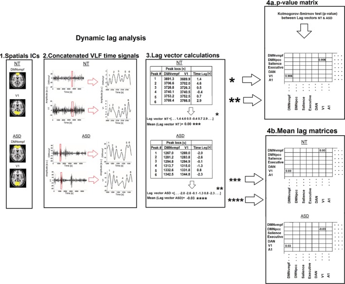
General workflow of dynamic lag analysis. (1) A given pair of resting‐state networks (RSNs) from the 16 RSNs is selected and (2) each peak of the time‐concatenated signals is determined with findpeaks function in MATLAB. (3) Next, the lag vector is formed by calculating the time lag values between each peak (between resting‐state networks) in the nearest neighbor principle (≤±5.0 sec lags). (4a) The Kolmogorov–Smirnov test is calculated between lag vectors of neurotypical and autism spectrum disorder to determine whether the lag variations are statistically different. (4b) The mean value of the lag vectors is calculated and assembled into a lag matrix. Steps 1–4 are applied to each selected resting‐state network pair separately to construct the final P‐value and mean lag matrices. Sections 4a and 4b are independent analysis phases.