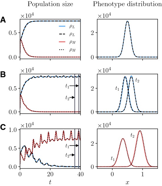
Fig. 3.

Left column. Plots of the population sizes ${\rho }_H(t)$ (red line) and ${\rho }_L(t)$ (blue line) obtained by computing numerically the integrals of the components of the numerical solution of the system of PDEs (3) subject to the initial condition (12). The dotted and dashed lines highlight, respectively, ${\rho }_H(t)$ and ${\rho }_L(t)$ obtained by solving numerically the Cauchy problem (14). The nutrient concentration S(t) is defined according to (79) with $M=1$ and $A=0$ (row a), $M=1$, $A=0.5$ and $T=5$ (row b), or $M=1$, $A=1$ and $T=5$ (row c)—cf. the plots displayed in Fig. 2. The values of the model parameters are those reported in Table 1 with ${\beta }_H=0.025$. Right column. Plots of the corresponding phenotype distribution of the surviving population obtained by solving numerically the system of PDEs (3) subject to the initial condition (12). In particular, the plot of $n_L(x,t_f)$ is shown in row a, while the plots in rows b and c are, respectively, those of $n_L(x,t)$ and $n_H(x,t)$ at $t=t_1$ and $t=t_2$, with $t_1$ and $t_2$ being highlighted in the corresponding plots in the left column. The dotted and dashed lines correspond to the exact phenotype distributions (13) with $v_i(t)$, ${\mu }_i(t)$ and ${\rho }_i(t)$ given by the numerical solutions of the Cauchy problem (14) (color figure online)