

Abstract
Osseointegrated (OI) prostheses are a promising alternative to traditional socket prostheses. They can enhance the quality of life of amputees by avoiding fit and comfort issues commonly associated with sockets. The main structural element of the OI prosthesis is a biocompatible metallic implant that is surgically implanted into the bone of the residual limb. The implant is designed to provide a conducive surface for the host bone to osseointegrate with. The osseointegration process of the implant is difficult to clinically evaluate, leading to conservative postoperative rehabilitation approaches. Elastic stress waves generated in an OI prosthesis have been previously proposed to interrogate the implant-bone interface for quantitative assessment of the osseointegration process. This paper provides a detailed overview of the various elastic stress wave methods previously explored for in situ characterization of OI implants. Specifically, the paper explores the use of electromechanical impedance spectroscopy (EIS) to assess the OI process in compress-type OI prostheses. The EIS approach measures the electrical impedance spectrum of lead zirconate titanate elements bonded to the free end of the implant. The research utilizes both numerical simulation and experimental verification to establish that the electromechanical impedance spectrum is sensitive (between 400 and 460 kHz) to both the degree and location of osseointegration. A baseline-free OI index is proposed to quantify the degree of osseointegration at the implant-bone interface and to assess the stability of the OI implant for clinical decision making.
Keywords: Prosthesis, Osseointegration, Electrical impedance spectroscopy, Guided waves, Bone, Piezoelectric
Introduction
The World Health Organization (WHO) estimates that there are over 30 million amputees worldwide [1]. To ensure amputees have a high quality of life, many rely on prostheses to replace their amputated limbs. The state-of-practice is the socket prosthesis which consists of a hard socket that covers the residual limb with an artificial limb mounted to the socket [2, 3]. While advances in socket prosthetic design have been made in recent years, there remains a number of drawbacks that can frustrate amputees to the point that they stop using the artificial limb [4]. For example, sockets can be difficult to perfectly fit to a residual limb leading to major discomfort and skin irritations including blistering and heterotopic ossification [5, 6]. In cases of extremely short or severely scarred limbs, the limb may not provide adequate surface conditions to accommodate a socket. Osseointegrated (OI) prostheses have been proposed as an alternative to socket prostheses, especially when socket prostheses are ruled out as a viable option. Advanced largely in Europe [7–10] and Australia [11] over the past two decades, OI prostheses are now beginning to be considered for greater use in the United States [5, 12].
OI prostheses are defined as prostheses that are surgically implanted into bone with one end extending transdermally out of the limb where an artificial limb is attached [13, 14]. To ensure long-term mechanical stability of the implant, implants are designed with a porous metallic surface that facilitates bone growth into the implant. OI prostheses offer many advantages including a direct load path from the artificial limb to the musculoskeletal system and osseoperception during limb use leading to dramatic improvement in amputee quality of life [12]. There are three major commercial OI protheses defined by different implant systems: screw implantation [e.g., Integrum’s Osseointegrated Prostheses for the Rehabilitation of Amputees (OPRA)], press-fit implantation [e.g., Permedica’s Osseointegrated Prosthetic Limb (OPL) and Orthodynamics’s Integral Leg Prosthesis (ILP)], and compress implantation using mechanical post-tensioning (e.g., Zimmer-Biomet’s Compress® Implants).
In the United States, Compress® Implants for OI prostheses are currently under study on a custom regulatory basis [5]. The advantage of the Compress® Implant is that it induces bone growth and remodeling over time due to the compressive forces it introduces into the host bone during implantation, resulting in stronger bone tissue capable of resisting higher loads [15, 16]. The design of the Compress® Implant is based on surgical insertion of a titanium anchor plug (Fig. 1) into the medullary cavity of the bone to offer a mechanically stable anchor to which a titanium spindle with a porous surface can be attached at the bone end. After the anchor has been inserted into the bone, transverse titanium pins are used to secure the anchor in place. The spindle is attached to the bone using small titanium screws that provide resistance to torsional loading. A threaded rod originating from the anchor plug and extending through the spindle is post-tensioned using nuts at the spindle end until a desired compressive axial force is applied to the bone between the anchor and the spindle. Several hundred pounds of compressive axial force are applied to stimulate bone growth and to accelerate the osseointegration process at the bone-spindle interface. Overtime, bone grows into the porous spindle surface as the bone tissue experiences increased density and stiffening (i.e., increased elastic modulus). Evidence of osseointegration is also the increased circumference of the bone at the bone-spindle interface (Fig. 2).
Fig. 1.
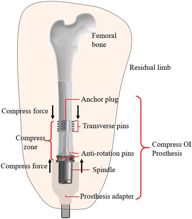
Conceptual diagram of a compress OI prosthesis in an adult femur
Fig. 2.
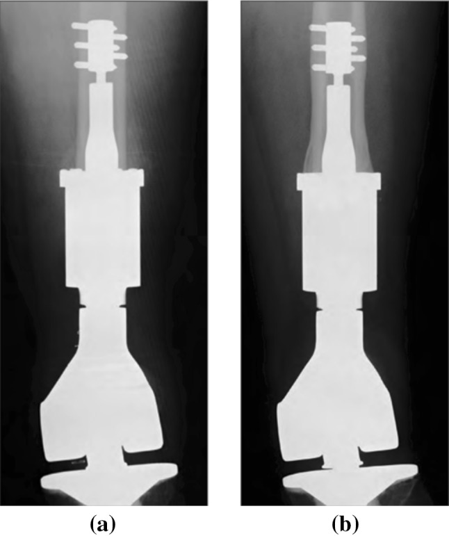
X-ray image of a Zimmer-Biomet Compress implant in adult femur: a day of the surgery; b 12 years after surgery with evident bone growth [21]
As OI implants grow in popularity, there is a need to improve patient outcomes including more efficient postoperative therapies and reduction of implant revisions [17]. Unfortunately, there remains a lack of clinical tools available that allow quantitative characterization of the condition of the bone-implant interface. Clinical evaluation of OI fixtures can be aided by X-ray radiographs but interpretation of radiographic images can be subjective and do not measure the mechanical attributes of the implant-bone interface [17, 18]. The example shown in Fig. 2 [19] demonstrates qualitative evidence of bone hypertrophy in a femur in which a Compress® Implant has been surgically implanted but it does not provide a direct measure of the degree of osseointegration. Especially in single-stage implantations, it can be difficult to clinically ascertain when the osseointegrated implant can be safely loaded. Premature loading can lead to long-term complications such as inadequate integration, implant loosening and periprosthetic fracture [17]. As a result, postoperative loading of the OI prosthesis is based on a conservative schedule derived from historical observation of healing in patients with a given type of implant. In general, postoperative therapies call for a multi-month period of gradual loading of the OI implant based on a defined loading schedule. Methods that can quantitatively measure the mechanical properties of the osseointegrated interface are highly desired to inform clinical loading protocols and to improve postoperative outcomes. These methods could also be used to clinically evaluate long-term complications that may develop including loosening of the fixture and the loss of osseointegration due to bone infection. A means of interrogating the prosthesis to ascertain the condition of osseointegration would be a powerful tool to making decisions centered on whether surgical revision is needed or not.
In this paper, a sensing strategy is proposed for clinical assessment of OI implants with a specific focus on compress-type OI implants. While the method presented is generalizable to other OI implant systems, the compress-type OI is selected because it is one of the implant designs being evaluated in clinical studies in the United States [5]. Emphasis is placed on developing a sensing system that resides outside of the body, thereby eliminating the need to develop sensing components that are biocompatible for safe use in the human body. Guided wave methods that utilize piezoelectric elements to generate elastic stress waves at the percutaneous end of the OI implant have shown great promise for interrogating bone-implant interfaces from outside the body. The paper begins with a summary of guided wave methods proposed for assessing osseointegration of implants ranging from dental implants to OI prostheses. Due to the unique geometric features of compress-type implants including the use of multiple mechanical components in the implant design, some of the previously proposed guided wave methods could be challenging to use. However, the electromechanical impedance spectroscopy (EIS) technique (also known as the electromechanical impedance (EMI) method) [20] is considered a good candidate for interrogating compress-type OI implants, especially for quantitative assessment of osseointegration that occurs at the bone-spindle interface. EIS methods measure the electrical impedance of piezoelectric elements bonded to the surface of the implant over a broad range of frequencies. Due to the electromechanical coupling between the piezoelectric and the implant, osseointegration of bone into the porous surfaces of the implant will manifest as changes in the impedance spectrum of the piezoelectric element. The study advances the EIS method for compress-type implants with piezoelectric elements bonded to the surface of the implant spindle. Numerical and experimental models are presented to validate the effectiveness of the EIS method in measuring the degree and spatial distribution of osseointegration using a baseline-free OI index that can quantify the degree of integration. Finally, the study explores the spatial sensitivity of the EIS method by varying the distance of piezoelectric elements relative to the osseointegration interface to define an interrogation zone for precise quantification of osseointegration by EIS. The paper concludes with a summary of key findings and a discussion on future work needed to further advance the work presented herein.
Background
Over the past three decades, sensing technologies have rapidly advanced resulting in high performing sensing solutions that can be used in a wide variety of biomedical applications ranging from wearable sensors measuring human activity [21] to in vivo sensors measuring glucose levels in blood [22]. More specific to orthopedic applications, guided wave methods have shown great promise. Initially developed in the field of structural health monitoring (SHM), guided wave methods use piezoelectric transducers mounted to a structure to launch elastic stress waves that can propagate across the structure; these propagating waves experience changes in wave properties that can be correlated to changes in the structure (i.e., damage) [23, 24]. In the case of biomedical applications, the structure interrogated by guided waves would be bones and implants [23, 24]. With guided wave sensing methods having the potential to interrogate OI prostheses using piezoelectric elements placed outside of the body, they represent a highly attractive monitoring strategy to consider.
Research has previously explored the use of elastic stress waves to interrogate and characterize the condition of human bones. In fact, ultrasonic waves have been widely used in the clinical assessment of osteoporosis [25]. For example, bone ultrasonometers are used to assess osteoporosis by stimulating ultrasonic stress waves in the calcaneus bone of a patient using a water-filled membrane attached to the heel as an actuator. The approach uses ultrasound centered at 500 kHz [26] to stimulate the bone to measure bone density. The low amplitude ultrasonic excitations inherent to these methods are proven to not be perceptible by human subjects.
A number of researchers have explored direct attachment of piezoelectric elements to bone to assess the condition of the bone. For example, Bhalla and Bajaj explored the use of PZT piezoelectric elements bonded to the surface of chicken femur bones for modal analysis [27]. Two PZT patches were mounted to serve as an actuator and sensor pair; the actuator was excited by a sinusoidal signal generating vibration in the bone with a “free-free” boundary condition. The excitation frequency was varied from 0.5 to 20 kHz to calculate the freqeuncy response function (FRF) from which the modal frequencies and damping ratios were extracted. These modal properties were shown sensitive to structural changes in the bone caused by drying and incision. Later, Bhalla and Suresh [28] expand on this initial work by using thin PZT elements bonded to a human femur using the EIS technique to quantify bone density. A root-mean-square deviation (RMSD) index was proposed to quantify changes in bone density. The piezoelectric elements were shown capable of also measuring fracture of the bone simulated by a cut introduced into the femur roughly 65 mm from the piezoelectric element. The impedance spectrum between 10 and 50 kHz showed distinct changes due to density change and bone fracture. More specific to OI prostheses, Vien et al. [18] proposed the integration of PZT elements directly into the design of a novel OI prosthesis that is 3D printed specific to the patient bone geometry. Their approach mounted four round PZT elements to the extramedullary struts of the 3D printed implant to stimulate and measure ultrasonic stress waves generated in the implant and that propagated into the bone. Input–output frequency response functions were generated between PZT actuator–sensor pairs with the power over a defined spectral bandwidth tracked during osseointegration. A scalar index was defined by the authors to aid in clinical decision making on the degree of osseointegration. A challenge of placement of ceramic sensing elements like PZT in the body is their lack of biocompatibility. To consider the body response to materials like piezoelectrics, Bender et al. [29] studied the use of piezoelectric elements implanted in soft tissue to characterize changes in the mechanical properties of the soft tissue. In a study population of 20 male Sprague–Dawley rats, implanted acrylic-coated PZT elements had detectable changes in their electromechanical impedance that correlated to soft tissue encapsulating the elements over time. Their conclusions state that challenges associated with the biocompatibility of piezoelectric elements must be resolved before they could be used inside the human body.
Alternatively, sensor placement outside of the body can be an effective approach to assessing the condition of bone healing and osseointegration of implants. Towards this end, pioneering work by Wong et al. [30] adopted external fixators used in the healing of fractured pelvis bones to stimulate the pelvis. The impact loading of one fixator at its free end transmitted vibrations into the fixated pelvis that allowed the pelvis response to be measured at a second fixator using PZT sensing elements attached to it. Measured PZT outputs were used to develop transfer functions of the pelvis which was shown sensitive to healing in the fixated pelvis. Ong et al. [31] later studied the changes in the FRF associated with a similar instrumented fixator set-up applied to a fully fractured femur bone. Fast cure epoxy was used to simulate bone healing with distinct changes in the FRF associated with this simulated healing scenario (i.e. epoxy curing). A unique feature of their work was that it also considered soft tissue effects by surrounding the femur bone model (i.e. sawbone) with modeling clay.
Specific to the external sensing of osseointegrated implants, Ribolla and Rizzo [32] explored the use of piezoelectric elements embedded in the exposed end of a dental implant to assess the osseointegration of the implants using electromechanical impedance techniques. Their work utilized a 3D numerical model built in ANSYS to simulate tissue healing condition of dental implants after surgery. The results of their study proved the EIS technique was sensitive to the postoperative healing of bone tissue around the dental implant with an impedance frequency of 565.5 kHz most sensitive to the degree of osseointegration. Similarly, Wang and Lynch [33, 34] proposed a quantitative approach to assessing osseointegration in OI implants using ultrasonic elastic guided waves. In their work, two circumferential PZT element arrays attached to the percutaneous surface of a solid titanium implant were used to excite longitudinal mode guided waves in the implant via tone burst signals. The results confirmed the energy of the longitudinal wave mode was very sensitive to osseointegration. Specifically, full osseointegration resulted in approximately 50% energy loss in the longitudinal wave mode reflected and sensed at the PZT array. In addition, the separation of the prosthesis from the bone was shown to significantly increase the energy received by the sensing piezoelectric array allowing for implant loosening to be identified. The approach by Wang and Lynch [33, 34] are well suited for OI implants consisting of monolithic solid rods because they rely on measurement and interpretation of propagating body wave signatures. These methods could be more difficult to apply to more complex OI implant systems like compress-type implants that consist of many components and interfaces. For this reason, this study considers an EIS approach to assessing osseointegration in compress-type OI implants because EIS methods do not require direct interpretation of waveforms propagating in the implant.
Materials and methods
In this study, a sensing strategy for the assessment of the osseointegration of bone into an OI prosthetic implant is presented. The method specifically adopts an approach of using instrumentation on the percutaneous end of the implant. Piezoelectric elements are selected to generate acoustic (i.e., 20 kHz or less) and ultrasonic (i.e., more than 20 kHz) elastic stress waves into the implant with the implant serving as a wave guide. The EIS approach [35] developed for SHM is adopted to explore wave frequencies most sensitive to the osseointegration process. While this strategy can be applied to most OI prosthesis types, the compress-type OI prosthesis is specifically considered in this study.
Electromechanical impedance spectroscopy (EIS)
Piezoelectric ceramic elements are proposed for installation on the percutaneous end of an OI prosthesis implant. Piezoelectric materials behave elastically when mechanically loaded as defined by Hooke’s law where is the strain field in the material, is the mechanical compliance matrix, and is the stress field in the material; they also exhibit linear electric behavior expressed as , where is the electric charge density, is the permittivity matrix and is the electric field strength vector [35, 36]. These behaviors are inherently coupled because the piezoelectric material generates a voltage when deformed (strained) and conversely will experience mechanical stress (strain) when an electrical field is applied. When considering this fact, a coupled set of equations for a piezoelectric element can be written assuming the application of constant electric, E, and stress, T, fields are applied,
| 1 |
where d is the matrix of the piezoelectric effect and is the converse piezoelectric effect [35, 36]. The electrical-based vectors and matrices of Eq. (1) have an associated coordinate system that align with the thin piezoelectric element where “1” and “2” define the plane of the element and “3” corresponds to the through thickness axis of the element. For example, the electric field in the “3” direction is denoted as E3. The mechanical-based vectors are indexed where S1, S2, and S3 are the strain fields in the 11, 22, and 33 directions, respectively. Similarly, S4 is the strain field in 23 direction, S5 is the strain field in 13 direction, and S6 is the strain field in 12 direction.
Now, consider a piezoelectric patch that is ideally (i.e., perfectly) bonded to the surface of a stiff host structure. When the piezoelectric patch is excited by a harmonic voltage in the “3” direction (i.e., through the element thickness), the patch experiences a mechanical stress and strain in the plane defined by the “1” and “2” directions. Conversely, when the element experiences strain in the “1” and “2” directions due to planar deformation of the underlying host structure, the piezoelectric element will generate a voltage field measurable in the “3” direction. The interaction model of the piezoelectric element bonded to the host structure under an electric excitation is demonstrated in Fig. 3.
Fig. 3.

Interaction model of a piezoelectric path bonded to a host structure under an electric excitation: a piezoelectric element set-up; b equivalent discrete element model
The EIS approach to interrogating a piezoelectric element is motivated by the fact that changes in the host structure will change the impedance of the element due to the mechanical coupling between the piezoelectric and the host structure. As shown in Fig. 3(b), the “host” structure can be modeled using discrete mechanical elements representing the mass, m (mp and mb for the mass of the prosthesis and bone, respectively), damping, C (Cp and Cb for the damping coefficient of the prosthesis and bone, respectively), and stiffness, K (Kp and Kb for the stiffness coefficients of the prosthesis and bone, respectively), of the bone and osseointegrated implant. As the osseointegration process evolves, the damping and stiffness of the bone at the implant surfaces will change. EIS will interrogate the PZT element attached to the implant using an electric field in the “3” direction by applying the voltage, , as a function of angular frequency, , with the current into the element, , simultaneously measured. The impedance, , of the piezoelectric element is then defined as .
The shear stress across the piezoelectric element-host structure interface in the case of ideal bonding is often simplified with a pin-force model [37]. Based on the interaction of the piezoelectric element-host structure modeled by Liang et al. [38], Dugnani et al. [39] and Bhalla et al. [35], the electromechanical admittance of the piezoelectric element can be represented in Eq. (2) as:
| 2 |
where is the admittance which is the inverse of impedance, . The admittance, , is complex valued and consists of real (i.e., conductance, G) and imaginary (i.e., susceptance, B) terms with j being the imaginary variable (). The measured admittance is dependent on the piezoelectric element geometry where l, w, and h is the half-length, width and thickness of the piezoelectric patch, respectively. Also,, is the complex electric permittivity at zero stress while denotes a dielectric loss factor. d31 and are the piezoelectric strain and electric permittivity constants at zero stress, respectively, which correspond to the 31 term of the piezoelectric effect matrix, d, and the 33 term of the permittivity matrix, , in Eq. (1), respectively. Finally, is the wave number of the PZT element, is the material density of the PZT wafer, is the complex Young’s modulus of the piezoelectric element under a constant electric field, and Zs and Zp are the mechanical impedance of the host structure and the PZT element, respectively. Zp can be expressed as:
| 3 |
The complex admittance can be decomposed into two parts: a passive component, , which is not affected by the structure, and an active component, , representing the coupled interaction between the host structure (i.e., implant and bone system) and the PZT element [28].
Compress-type OI prosthesis
Unlike other OI implants, the compress-type OI prosthesis fixture introduced by Zimmer-Biomet [17, 19] uniquely utilizes a compression mechanism during surgical implantation that is designed to stimulate continuous axial load on the host bone to induce bone growth according to Wolff’s law. The compress OI device is designed to have a mechanical anchor plug that is implanted in the intramedullary channel of the bone with a threaded rod axially extending past the bone. A spindle with a porous titanium surface is attached to the end of the bone with nuts screwed onto the anchor rod to affix the spindle to the bone; tightening the nut controls the compressive axial force applied to the bone via post-tensioning of the threaded rod. The spindle is also stabilized using three anti-rotation screws surgically implanted into the bone (Fig. 1). Typically, between 400 and 800 lb of axial compressive force is imposed on the bone during surgery. Osseointegration occurs on the bone-spindle interface accelerated by the constant axial compression on the bone. Concurrent to bone growth into the porous titanium spindle surface, the diameter of the bone increases.
The compress-type OI implant system designed for this study is similar to the commercial Compress® implant from Zimmer-Biomet and contains six parts (Fig. 4): (1) a titanium anchor plug with a post-tension rod, (2) five titanium transverses pins that attach the anchor plug to the bone, (3) three anti-rotation pins that stabilize the spindle, (4) titanium spindle, (5) locking cap, and (6) nut. The anchor plug and rod are machined from solid titanium (Grade 5) that is 150 mm long with a 12 mm diameter plug machined in the top 30 mm and a 10 mm diameter rod machined over the remaining 120 mm length. The lower 25.6 mm of the rod is machined to have 22 threads per inch (8.7 threads per cm). The anchor plug is slipped into the interior of the host bone after the intramedullary channel of the bone is reamed with a diameter 12 mm or greater. Five 2 mm diameter transverse holes are included in the top of the anchor rod. A drill guide that templates the hole locations in the anchor plug is used to drill five holes in the bone in locations that align perfectly with those in the rod. Five transverse titanium pins (also with 2 mm diameter) are then press fit into the bone and through the corresponding holes in the anchor plug to secure it in the bone. The spindle is also made from titanium with a flat but roughened top surface. The top surface has a 42 mm diameter and has three holes that allow titanium screws to screw into the bone to stabilize the spindle when attached to the bone end. A titanium locking cap with a 42 mm diameter connects to the spindle. The threaded end of the anchor rod is exposed after the spindle and locking cap have been placed against the bone end; a titanium nut screwed onto the threaded rod is used to compress the bone. To assess the axial force applied to the anchor rod and bone, a specific chamber is designed in the spindle for the placement of a metal foil stacked rosette of strain gauges (Micro-Measurements 062WW) with nominal resistances of 350 Ω and gage factors of ζ = 2.14. The rosette is intended only for measuring the axial compression in the bone during experimental testing and is not being proposed for use in real OI prostheses implanted in human subjects. The details of each part are shown in Fig. 4. The implant components are made from solid isotropic titanium (Grade 5) whose density, , is 4330 kg/m3, modulus of elasticity, E, is 110 GPa, and Possion ratio is 0.33.
Fig. 4.

Design of a compress-type OI prosthesis implant for implantation in a human femur (as shown in Fig. 1)
A total of nine PZT piezoelectric elements (4 mm × 4 mm × 0.5 mm) sourced from Piezo Systems (Type 5A4E) are selected to be the electrical impedance sensors to assess osseointegration on the spindle-bone interface. Six of the PZT elements are bonded to the side of the spindle where the spindle has a 24 mm diameter neck (see Fig. 4). The neck of the spindle is machined to offer square flat surfaces (4 mm by 4 mm) on the external surface to provide six equally spaced flat surfaces on the spindle circumference for the placement of piezoelectric elements. In order to investigate the sensitivity of the EIS method to PZT element placement, the remaining three PZT elements constitute another circumferential array which is 20-mm below the spindle neck and further away from the bone-spindle interface. Also equally spaced, three square surfaces (4 mm by 4 mm) are machined to offer flat surfaces for the PZT elements. All piezoelectric elements are attached to the spindle surface using cyanoacrylate glue (fully cured glue with a density of 1250 kg/m3 and the elastic modulus of 3.5 GPa).
A synthetic sawbone (Sawbones Worldwide Model 3406-5) is selected as the host femoral bone for implantation of the compress-type OI prosthesis. This surrogate bone model is made from solid rigid polyurethane with a density, , of 1600 kg/m3. The biomechanics properties of the sawbone are intended to be close to those of an adult femur bone. The bone is reamed with a 18 mm-diameter hole in the interior intramedullary cavity. In addition, five holes with a diameter of 2 mm are drilled at the range of 50-70 mm from the bone implant end to place the transverse pins used to stabilize the anchor plug placed in the reamed intramedullary bone cavity. The assembled compress-type OI prosthesis implanted in the femoral sawbone is shown in Fig. 5.
Fig. 5.

Fully assembled compress-type OI prosthesis implanted in femoral sawbone model
Numerical OI prosthesis-bone model
In addition to the physical OI prosthesis-bone model used in the laboratory, a finite element method (FEM) model (Fig. 6) is developed to consider a broader range of scenarios including the development of osseointegration after implantation and sensitivity analysis of the PZT element location relative to the spindle-bone interface where osseointegration occurs. An accurate three-dimensional geometric model of the femoral sawbone bone is created by using an optical camera and 3D laser scanner as previous described by Wang and Lynch [34]. The complex 3D model of the femoral bone is imported into ABAQUS, a commercial FEM software platform.
Fig. 6.

OI prosthesis-bone model: a compress-type implant in femur bone model; b meshing used in ABAQUS
The FEM model is divided into four major parts each with its own model parameters: femur bone, OI compress device, piezoelectric elements, and intramedullary bone tissue with adjustable material properties that correlate to osseointegration. As shown in Fig. 6b, each component is mapped in different colors to highlight the different model parts: the bone is modeled using grey elements, the titanium OI prosthetic device using cyan elements, the piezoelectric elements using red elements, and the adjustable intramedullary tissue using pink elements. A circular blind hole with a diameter of 18 mm and a depth of 80 mm is created from the implant end of the bone to simulate reaming during surgery [40]. A flat-top cone whose longitudinal axis is aligned with the longitudinal axis of the bone is created at the spindle end of the bone to simulate bone hypertrophy caused by compression delivered by the implant. The top radius of the cone is 10 mm, the height of the cone is 10 mm, and the bottom radius of the cone is varied from 10 to 20 mm with a step of 2 mm according to the degree of integration which will range from 0 to 100% with a step of 20%. It should be noted that the bone cross section is not perfectly circular and has a complex geometry; the flat-top cone therefore is superimposed in space with the bone with the geometry of the flat-top cone and bone merged to create solid structural (bone) assembly (also shown in Fig. 14a). The machined femoral bone is meshed by a 10-node quadratic tetrahedron 3D stress element (C3D10) with a 1 mm sizing seed resulting in a total of 25,956 elements. As a typical anisotropic material, the orientation of the bone is defined in a cylindrical coordinate system. The material properties of the femoral bone modeled in ABAQUS are listed in the Table 1 according to standard biomechanical references [41, 42].
Fig. 14.

a Circumference PZT arrays at different distances from the spindle top; b changes in normalized OI index for experiment and simulation
Table 1.
| Mechanical parameters | Longitudinal direction | Orthogonal directions |
|---|---|---|
| Elastic modulus (GPa) | 16.0 | 6.8 |
| Shear modulus (GPa) | 3.6 | 3.3 |
| Poisson ratio | 0.45 | 0.3 |
| Density (kg/m3) | 2000 | 2000 |
The compress-type OI device model is created based on the implant components including the anchor plug and post-tension rod, five transverses pins, spindle, and locking cap. The anti-rotation pins are neglected due to the spindle not being loaded in torsion in the analysis. Also, the nut is neglected in the model because an external force will be applied directly to the locking cap and anchor rod to simulate compression on the bone. The overall dimension of the compress-type implant is the same as the design described in Fig. 4. Because of the irregular geometry of the implant, a 4-node linear tetrahedron 3D stress element (C3D4) is employed to mesh the implant. A total of 12,135 elements are generated to model the implant including 1762 elements for the locking cap, 8828 elements for the spindle, 825 elements for the anchor plug and rod, and 144 elements for each transverses pin. The property of each part of the compress-type OI device is titanium, a typical isotropic material, whose density, , is 4500 kg/m3, Young’s modules, , is 11.0 GPa, and Possion’s ratio, , is 0.33.
The intramedullary bone tissue between the anchor plug and spindle will be affected by the compressive forces introduced in the bone and osseointegration between the bone and the porous surface of the spindle. This process requires the ability to vary the properties of the intramedullary tissue. The tissue in this region has both the inorganic (minerals) and organic (collagen) components [43]. The mechanical properties of the tissue depend on the mineral constituents (calcium and phosphate) that offer the bone load bearing capacity and the collagen providing the bone with flexibility. According to Manjubala et al. [44], the density () and elastic modulus (Ebone) of adult bone increases with a change of mineral content associated with the osseointegration process. Thus, to simulate changes in the intramedullary bone properties due to the compressive load, a script written in Python is used to randomly select the finite elements in the intramedullary tissue to form eight groups. As described by Wang and Lynch [34], eight groups allow the modulus and density of each element to have a random spatial variation of ± 2% from the mean value. The mean density () and elastic modulus (Etissue) is increased from 0% to 100% with a step of 20%. Initially the intramedullary tissue is assumed to have a density of = 1 kg/m3 and modulus of Etissue= 1 kPa (corresponding to 0% osseointegration). At each step of osseointegration (20%) the density and modulus increase by 400 kg/m3 and 3.2 GPa, respectively. At 100% osseointegration, the final density is 2000 kg/m3 and modulus is 16 GPa.
Piezoelectric elements are modeled from lead zirconate titanate (PZT) ceramic materials with a size of 4 mm (length) × 4 mm (width) × 0.5 mm (thickness). The properties of the piezoelectric elements are provided by the manufacturer, Piezo Systems, and listed in the following equations:
| 4 |
| 5 |
| 6 |
The 8-node linear piezoelectric solid brick element (C3D8E) is used to mesh each PZT element with a 0.2 mm sizing control seed resulting in each element containing 800 elements. The element size must be half of the smallest wavelength of the wave modes propagating in the model or smaller (in this case, 0.2 mm is much less than 0.5 where is approximately 3 mm based on the EIS frequency range adopted in the following section) to accurately capture the response of the PZT element [45]. The stiffness matrix, CE, piezoelectric coefficient matrix in strain form, d, and dielectric constant matrix, are converted to follow the ABAQUS order represented in Eqs. (4), (5) and (6). Each PZT element is bonded to the surface of the spindle with a series of “tie” constraints created in the “interaction” section. The master surface is the bottom surface of the PZT element and the slave surface is the top surface of the titanium spindle. In addition, tie constraints are also employed to unite the femur, intramedullary tissue, and implant together.
Results
Pristine PZT element impedance
The PZT element used in the numerical model must be calibrated to correspond to a real PZT element tested in the laboratory. In this step, a PZT element in free space is modeled and later tested using the EIS method of sweeping the electrical excitation frequency over which impedance is measured. First, the PZT element (4 by 4 by 0.5 mm3) previously described is modeled alone in ABAQUS as shown in Fig. 7. To account for damping in the piezoelectric, stiffness proportional damping is assumed to introduce a form of dissipative energy loss during straining; a proportionality constant of 2 × 10⁻⁸ is used according to Nader et al. [46]. In ABAQUS, a harmonic voltage, , with a V0 = 1 V amplitude is applied to the top surface of the PZT element with the frequency of the harmonic varied; the bottom surface of the PZT element is grounded. A “steady-state dynamics, direct” analysis step is created with linear scale to compute the response of the PZT element. The frequency range of excitation is varied from 2 kHz to 1000 kHz with an increment of 2 kHz.
Fig. 7.

Numerical model and excitation-response schematic of pristine PZT element
The impedance of the PZT cannot be directly extracted from the finite element model. Rather, the impedance of the PZT element will be calculated based on the surface charge value of the PZT element. A boundary set is created on the top surface of the PZT element to capture the reactive electrical nodal charge in the field output. The real and imaginary terms of the reactive electrical nodal charge of the top PZT surface is saved for each voltage excitation. The reactive electric charge of the top surface of the piezoelectric element is calculated from an integral applied to the entire top surface of the element in both the x- and y- dimensions as shown:
| 7 |
where qI and qR are the imaginary and real terms of the charge, respectively, q(x, y) is the reactive electrical nodal charge at the location (x, y), and is the integral region of the top surface. In the post-processing stage, the impedance and admittance of the piezoelectric element is calculated based on the relationship between the excitation voltage, V, and the reactive surface charge, Q. The value of the current flow, , is equal to the charge times the angular frequency of the excitation, :
| 8 |
Then the electromechanical admittance, , and impedance, , of the PZT element is computed:
| 9 |
| 10 |
Meanwhile, the impedance of the real PZT elements are measured prior to placement on the compress-type OI implant. To experimentally measure impedance, an impedance analyzer (Agilent 4284A Precision Impedance Analyzer) is employed to measure the complex admittance value of the PZT element. Copper foil tape with a conductive adhesive is attached to the top and bottom surface of the PZT element. Copper tape is an ideal approach to attaching electrodes to the PZT element because it is not stiff and will not mechanically impede the free vibrations of the PZT element. The programed frequency range is set from 1 to 1 MHz which cover the first three vibration modes of the PZT (according to the simulation results) with a linear frequency sweep. The applied voltage amplitude is 1 V which is identical to the simulation harmonic excitation amplitude. A total of 801 measurement points are equally distributed in the frequency span with the measured complex-valued admittance of the piezoelectric element saved. At each point, the real term conductance, G, and the imaginary term susceptance, B, are averaged eight times to cancel measurement noise.
Figure 8a shows a comparison of the PZT admittance spectrum measured by the impedance analyzer and that simulated by ABAQUS. In the numerical simulation results, there are three admittance peaks in the spectrum: 431.2, 626.0, and 905.2 kHz. In the experimental results, the first two peaks are clearly observed at 431.2 kHz with a value of 8.9 mS and the other at 626.0 kHz with a value of 0.9 mS. The last peak is barely observed because it has a much smaller value than the first two peaks. The electromechanical impedance results of the PZT in experiment and simulation are demonstrated in Fig. 8b. There are five peaks at 430.6 kHz, 520.5 kHz, 616.6 kHz, 640.4 kHz, and 906 kHz, respectively, in the impedance curve. The experimental results validate the resonant frequencies of the pristine PZT element as modeled in simulation. As we can see, both the admittance and impedance measured by the analyzer have good agreement with the computed results captured by the numerical simulation. While the peak admittance and impedance amplitudes from the simulation tend to be higher, the damping used in the simulation was selected to minimize discrepancies in peak frequencies between model and experiment. None the less, the strong agreement between the model and experiment validates the simulation environment as a reliable alternative to extensive experimental testing.
Fig. 8.

Comparison of the experimental and simulated results of pristine PZT element: a admittance; b impedance
Experimental impedance monitoring during the compression process
According to Zimmer-Biomet [19], the compress-type OI device should be loaded 400 (1780 N) to 800 lbs (3560 N) of axial compressive force by tightening the nut to create a compress zone that is intended to accelerate the healing process. To investigate if the level of compression in the bone affects the electromechanical impedance measured by the PZT elements, the impedance of the surface mounted PZT on the spindle are measured for specific axial compression levels. In the laboratory, the rosette strain gauge glued on the surface of the titanium post-tension rod is employed to ensure the axial compressive force is set to 400 lbs, 600 lbs, and 800 lbs with electrical impedance of a PZT element measured for each compressive load.
A Wheatstone bridge circuit is developed to measure the tension strain of the anchor rod from which the tensile force, F, is estimated by,
| 11 |
| 12 |
where is the strain measured by the rosette strain gauge through a half Wheatstone bridge applied on the tension rod, is the stress in the rod calculated from the tension strain, and are the Young’s modulus and Poisson ratio of titanium, D = 10 mm is the diameter of the titanium anchor rod, 2.14 is the gauge factor provided by the manufacturer, UA is the bridge output voltage (measured by a standard laboratory data acquisition unit), and UE is the bridge input voltage or excitation voltage which in this study was set to 12 V as delivered by a stable DC power supply (Agilent E3642A DC power supply).
The aforementioned impedance analyzer (Agilent 4284A) is utilized to measure the electric complex admittance value of the PZT element during the loading process. As shown in Fig. 9, after the PZT is attached to the implant spindle, the resonant peaks of the implant and PZT element are captured in the EIS results. The maximum peak in the admittance curve drops from 8.9 (Fig. 8a) to approximate 6.5 mS accompanied by a shift from 431.2 to 448.0 kHz. In addition, a new resonant peak at 381.8 kHz is seen in the admittance spectrum (Fig. 9a) which is attributed to the implant. The admittance and impedance of the pristine PZT element measured in the previous experiments are plotted using a gray dotted line as a reference. Similarly, Fig. 9b shows the measured impedance value of the PZT element during compressive loading of the bone. Similar to admittance, the impedance peaks of the PZT shift to the right after being attached to the spindle. Also, the new resonant frequency of 381.8 kHz is also observed in the impedance spectrum. Perhaps the most important finding is that neither admittance nor impedance show any change as a result of compressive loading. This result suggests the EIS method is insensitive to the compression force making its use in clinical setting easier to generalize should patients have different compressive forces applied.
Fig. 9.

Experimental EIS results of the compress OI device with loading force: a admittance; b impedance
Experimental and numerical simulation of impedance change during osseointegration
To mimic the osseointegration process that will occur between the bone and spindle surface in the laboratory, a 30-min slow-cure epoxy is injected into the gap between the spindle and the sawbone with the bone in axial compression of 800 lbs. This 30-min epoxy adhesive has a fully cured elastic modulus of 3.5 GPa and a density of 1550 kg/m3, which are relatively close to that of the soft intramedullary tissue. According to previous research [34], this epoxy is well-qualified for simulating the osseointegration process. The impedance analyzer is used to measure the conductance and susceptance of each PZT element bonded to the spindle every 6 min up till 30 min of cure time. In addition, EIS measurements are also take at 45 min and 60 min after epoxy injection to make sure the epoxy is fully cured. The measurements are taken eight times and averaged to cancel noise in the EIS measurements.
As can be seen in Fig. 10, both the admittance and impedance of the PZT element changes significantly during epoxy curing, which indicates the EIS method is sensitive to the simulated osseointegration of the bone into the spindle surface. Both the electrical impedance amplitudes and resonant frequencies appear to correlate to the degree of simulated osseointegration. The greatest changes in conductance and impedance appear to be in the frequency range 400–460 kHz, which could be used to derive an index to track the osseointegration process. Figure 11(a) present a close-up view of the conductance signature in the range of 400–460 kHz. As can be seen, the peak value of conductance decreases from 6.3 to 3.2 mS at the peak frequency of 449.2 kHz during curing (which is a surrogate for the osseointegration process). Meanwhile, the value of conductance at the EIS resonant frequency 393.1 kHz (the resonant peak corresponding to the implant) increases with the cure time (osseointegration). As we can see from Fig. 10b, the impedance value at 449.2 kHz also indicates the structural impedance increases with the osseointegration process.
Fig. 10.

Experimental EIS results of the osseointegration of prosthesis-bone interface: a admittance; b impedance
Fig. 11.

Conductance signature of PZT element 1 at various osseointegration stage: a experiment; b simulation; c OI index based on the experimental data; d OI index based on the numerical data
In the numerical model, an 800 lbs (3560 N) compressive axial force is applied on the locking cap while 800 lbs (3560 N) of tensile axial force is applied to the rod. The osseointegration simulation starts from 0% osseointegration with the elastic modulus and density of the intramedullary tissue set to 1 kPa and 1 kg/m3, respectively, in ABAQUS. The flat-top cone is also set with a bottom radius of 10 mm. The EIS approach is simulated with the PZT impedance spectrum calculated. Next, the average density () and elastic modulus (Etissue) of the intramedullary tissue increase from 0 to 100% with a step of 20% (i.e., density and modulus increments of 400 kg/m3 and 3.2 GPa, respectively). The numerical simulation focuses on the signature frequency range (400–460 kHz) to shorten the computational time. The simulated conductance for each step of osseointegration is shown in Fig. 11b. The simulation results of PZT admittance is in good agreement with the experimental EIS results captured by the impedance analyzer during various osseointegrated stages in the laboratory (see Fig. 11a).
In the application of the EIS method in SHM, the RMSD index [20] is widely used to describe a change of PZT conductance signature due to changes in the host structure such as damage; the RMSD method depends on a pre-damage baseline. In addition, the RMSD is often calculated at specific resonant frequencies. In the results presented for the compress-type OI implant, it is clear that more than one peak is influenced by osseointegration. Hence, this work seeks to establish a baseline-free osseointegration (OI) index to quantify the degree of osseointegration. As established by Ribolla and Rizzo [32], the amplitude of conductance decreases at the signature peak frequency while the amplitude of conductance increases at its neighboring non-peak frequencies. In other words, the osseointegration is akin to increasing damping at the spectrum peak, resulting in a smoothing process of the conductance peak. Thus, a novel baseline-free OI-index is defined as,
| 13 |
where Gi is the conductance at discrete frequency, G is the averaged conductance value in the signature frequency range,
| 14 |
and n denotes the total number of discrete frequencies in the signature range. As previously stated, the signature frequency range is from 400 to 460 kHz which involves 48 discrete frequencies in the experimental data and 31 discrete frequencies in the simulation. The OI indexes are calculated according to Eq. (13) for both the experimental and numerical EIS data to assess the state of osseointegration as shown in Fig. 11c, d. Figure 11c shows the OI index of the experimental data (with epoxy serving as a surrogate to osseointegration) has a sigmoidal shape with increasing OI index with degree of the osseointegration; similar sigmoidal changes in curing epoxy properties are observed by Love et al. [47] and Dümichen et al. [48]. The OI index of the numerical data (Fig. 11d) is relatively similar to the experimental data but with a more consistent linear quality. The results validate the functionality of the proposed OI index. It is emphasized that the OI index is a baseline-free index which is independent of the original state immediately after surgery. As a result, it could serve as a convenient index for clinical applications which may have the EIS method applied to the OI prosthesis at any period after surgery (and not necessarily at the instant of implantation).
Impedance monitoring for periprosthetic fractures
Periprosthetic fracture can occur at the interface of compress-type OI implants and their host bones generally caused by improper usage or accidents [17]. When periprosthetic fractures occur, implant revision is necessary including the resection of bone and additional internal fixation. To address this failure mechanism in compress-type implants, the EIS method is proposed for monitoring periprosthetic fractures. Numerical simulation is more suitable than experimental testing to validate the feasibility of the proposed EIS approach and corresponding OI index to observe localized failure of the osseointegration surface. Also, the work will inform understanding of how spatial variation in the osseointegration process can be observed with the PZT elements bonded to the implant spindle.
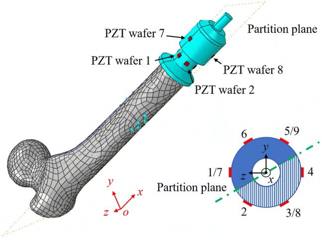
Since periprosthetic fractures often cause disruption to the bone-prosthetic interface according to the study of Wakenda et al. [17], the osseointegration interface on the spindle top surface is partitioned into two different sections by a datum plane in ABAQUS: half of the tissue is set to be fully osseointegrated, and the other half of the tissue is set to have a decreasing degree of osseointegration from 100 to 0% with a step of 20%. Again, 800 lbs (3560 N) of compressive force is applied to the bone. The partition plane of the two halves is selected to be 30 degrees to the xoz plane in order to keep the integrity of all the PZT elements (see Fig. 12). The boundary is set such that half of the section is on the side of PZT elements 2, 3, 4 and 8 (partial osseointegration) and the other is on the side of PZT elements 1, 5, 6, 7 and 9 (fully osseointegrated). The impedance of the PZT elements in the signature frequency range will be calculated via simulation.
Fig. 12.
Numerical model with two halves tissue partitions
As can be seen in Fig. 13a, the normalized OI index of all nine PZT elements decrease with the decreasing degree of osseointegration on half of the osseointegration surface at the spindle top. The OI index of the first circumferential array (PZT 1, 2, 3, 4, 5, and 6) decrease more than the second array (PZT 7, 8, and 9) which indicates the circumference of PZT elements closest to the spindle top are generally more sensitive to the osseointegration condition. For this first circumferential array, the OI index of the three PZT elements closest to the changing osseointegration half (PZT 2, 3, and 4) are most sensitive to changes significantly dropping approximately to levels between 55% to 72% of the original OI index. The other three PZT elements (PZT 1, 5, and 6) on the side of the fully osseointegrated portion have index values decreasing much less to values of 86–92% of the original OI index. Especially, the OI index of PZT element 3 reduces the most from approximately 55% of the original index because it is in the center of the closest circumferential PZT array in the half section with reducing osseointegration. Similarly on the second circumferential array, the OI index of PZT 8 which is in the half section with reducing osseointegration decreases more than that of PZT 7 and 9. In summary, the results validate the proposed OI index is sensitive to the osseointegrated state while also showing spatial variability correlated to the location of osseointegration. This suggests the EIS approach, when applied to PZT arrays around the circumference of the OI implant, can provide insight to the spatial properties of osseointegration while also holding promise for the early identification of periprosthetic fractures.
Fig. 13.

a OI index of the numerical modal with half tissue decreasing osseointegration; b OI index of the experimental with solidifying of half epoxy
For experimental testing, the compress-type OI prosthesis implant is again inserted into a sawbone. After compressive load is applied (800 lbs (3560 N)), epoxy is injected into an area between the bone and spindle over roughly half of the section. After multiple hours of curing, the second half of the bone-spindle interface has epoxy injected with the EIS method applied in using the protocol previously described (EIS measurements of the PZT elements taken every 6 min up until 30 min and then at 45 and 60 min). After averaging the admittance measurement of each PZT element eight times for denoising (takes about 30 s), the impedance analyzer is connected to the next element for measurement. The PZT locations are identical to that shown in Fig. 12. The normalized OI index of the PZT conductance in the signature frequency range are shown in Fig. 13b. As can be seen, the proposed OI indexes of all the PZT elements increase with cure time in the expected sigmoidal fashion. Especially for PZT 3 (the PZT element closest to the curing epoxy half section), the OI index significantly increases from 0.56 to 1 during the cure time. In addition, the OI indexes of PZT 2, 3, and 4 closed to the solidifying epoxy increase more than the other six PZT elements. Finally, the averaged OI index of the second circumferential array of PZT elements increases less than that of the first array in spite of PZT 8 increasing more than PZT 5.
EIS sensitivity to distance to osseointegration
To explore the sensitivity of the PZT element to the distance from the osseointegration site, four circumference arrays of PZT elements are created and bonded at various locations on the implant spindle in the numerical model. As shown in Fig. 14a, each array contains six PZT elements on the spindle circumference: the four arrays are attached 9.5 mm, 19.0 mm, 38.0 mm, and 56.0 mm, from the end of the bone in contact with the spindle. The density () and elastic modulus (Etissue) of the intramedullary tissue is modeled with 0–100% degree of osseointegration in ABAQUS. The normalized difference in the OI index between the 0–100% osseointegration cases are calculated for each PZT element and plotted in Fig. 14b. The difference in normalized OI index of the PZT elements simulated in ABAQUS are plotted as red dots in Fig. 14b along with statistical characteristics (mean values and standard deviations) plotted as black bars. Evident is that the mean value of the difference in OI index significantly decreases (from 0.74 to 0.10) with increasing distance between the osseointegration surface and the PZT circumferential array. The results show that the closer the PZT elements can be placed to the osseointegration interface, the more sensitive the OI index is to measuring osseointegration. Thus, to obtain results in a clinical setting, the PZT elements should be attached as close as possible to the osseointegration zone.
Conclusions and discussion
In this study, a quantitative approach to clinical decision making centered on the osseointegration of OI prostheses was proposed. The EIS approach was explored using PZT piezoelectric elements attached to the implant for the generation of acoustic and ultrasonic waves in the implant. A laboratory model was developed consisting of a femoral sawbone and a compress-type OI device whose design was inspired by the commercial Compress® implants developed by Zimmer-Biomet. An identical numerical model was also developed in ABAQUS for simulation of the OI implant system. Nine PZT elements bonded to the surface of the implant spindle and whose electrical impedances were measured were shown sensitive to changes simulated at the implant-bone interface. In the experimental model, slow-curing epoxy was used at the bone-spindle interface to simulate osseointegration while in the numerical model, the properties of the intramedullary tissue were changed in a manner consistent with tissue stiffening and densification during osseointegration. Overall, the EIS method proved to be sensitive to osseointegration in the compress-type OI implant while simultaneously being insensitive to the magnitude of compression introduced in the bone during implantation. As osseointegration occurred, the peak value of conductance at a resonant frequency of 449.2 kHz decreased while the impedance value at this frequency increased. The conductance spectrum of the bonded PZT element in the range of 400–460 kHz also changed. A baseline-free OI index was defined based on the conductance spectrum over this signature band. Similar results were found during experimentation using epoxy to simulate osseointegration in the laboratory. The quality of the data associated with the EIS method was proven to be dependent on the location of the PZT elements with elements closest to the osseointegration surface more sensitive to osseointegration. Finally, the EIS method showed spatial sensitivity to osseointegration with the spatial distribution of osseointegration detectable based on the location of PZT elements on the spindle circumference. These findings offer promise for use of the EIS method to identify periprosthetic fractures. The EIS method presented in this study can be generalized to other implant types including screw- and press fit-type implant systems as other studies have suggested [32]. To apply the method to these other implant-types, studies would need to be performed to assess the sensitivity of piezoelectric element impedance to osseointegration as a function of the element distance from the osseointegration interface. Similarly, a spectral region of the piezoelectric impedance function sensitive to osseointegration would need to be identified.
While the study shows great promise for the EIS method in clinical evaluation of osseointegration in OI prosthesis implants, some limitations are also evident. In this study, only one bone model was considered. It is anticipated that variations inherent to a population of patients receiving OI implants will have to be considered including differences in bone geometries, bone properties, and implantation technique, just to name a few. Also, this study did not consider how the method can be applied to the transdermal adapter that attaches to the implant spindle and that presents the percutaneous end where instrumentation can be installed. While the study highlighted the sensitivity of the EIS method to osseointegration in compress-type OI implants, additional research is needed to assess the selectivity of the method to osseointegration to ensure other factors could not affect impedance values that would lead to incorrect conclusions in a clinical setting. For example, changes in the soft tissue surrounding the bone and transdermal adapter would need to be studied to assess EIS spectral regions sensitive to osseointegration are not affected. These limitations and open questions should guide future work. Towards this end, future clinic study is needed to evaluate the EIS method on amputees with OI prostheses. In such a clinical setting, different implant systems can be considered including compress-type OI implants. Clinical evaluation would allow variations in bone properties and the effects of soft tissue to be explored over a population of subjects. In a clinical study, the EIS method would bond the PZT elements to the percutaneous end of the transdermal adapter. This would allow for optimization of the design of the PZT array (i.e., size and location) and the selection of the excitation signal to maximize the sensitivity of the EIS method to osseointegration occurring on the spindle attached to the adapter. Also, human perception of the elastic waves being generated in the implant could be assessed.
Funding
This study is financially supported by the Office of Naval Research under Grant N00014-18-1-2477. The authors also wish to acknowledge the guidance provided by Dr. Liming Salvino (Office of Naval Research) and Dr. Jonathan Forsberg (Walter Reed National Military Medical Center).
Compliance with ethical standards
Conflict of interest
The author declares that there is no conflict of interest regarding the publication of this paper. The compress-type OI implant system presented in this study is similar to the commercial Compress® implant from Zimmer-Biomet but was independently designed and manufactured by the paper authors. The authors have no financial relationship with Zimmer-Biomet.
Ethical approval
This article does not contain any studies with human participants or animals performed by any of the authors.
Footnotes
Publisher's Note
Springer Nature remains neutral with regard to jurisdictional claims in published maps and institutional affiliations.
References
- 1.World Health Organization. Guidelines for training personnel in developing countries for prosthetics and orthotics services. https://apps.who.int/iris/bitstream/handle/10665/43127/9241592672.pdf.
- 2.Ziegler-Graham K, MacKenzie EJ, Ephraim PL, Travison TG, Brookmeyer R. Estimating the prevalence of limb loss in the United States: 2005 to 2050. Arch Phys Med Rehab. 2008;89(3):422–429. doi: 10.1016/j.apmr.2007.11.005. [DOI] [PubMed] [Google Scholar]
- 3.Fischer, H. A guide to US military casualty statistics: operation freedom’s sentinel, operation inherent resolve, operation new dawn, operation Iraqi freedom, and operation enduring freedom. https://fas.org/sgp/crs/natsec/RS22452.pdf.
- 4.Paternò L, Ibrahimi M, Gruppioni E, Menciassi A, Ricotti L. Sockets for limb prostheses: a review of existing technologies and open challenges. IEEE T Bio-Med Eng. 2018;65(9):1996–2010. doi: 10.1109/TBME.2017.2775100. [DOI] [PubMed] [Google Scholar]
- 5.McGough R, Goodman M, Randall R, Forsberg J, Potter B, Lindsey B. The Compress® transcutaneous implant for rehabilitation following limb amputation. Der Unfallchirurg. 2017;120(4):300–305. doi: 10.1007/s00113-017-0339-9. [DOI] [PubMed] [Google Scholar]
- 6.Herbert N, Simpson D, Spence WD, Ion W. A preliminary investigation into the development of 3-D printing of prosthetic sockets. J Rehabil Res Dev. 2005;42(2):141–146. doi: 10.1682/JRRD.2004.08.0134. [DOI] [PubMed] [Google Scholar]
- 7.Brånemark R, Berlin Ö, Hagberg K, Bergh P, Gunterberg B, Rydevik B. A novel osseointegrated percutaneous prosthetic system for the treatment of patients with transfemoral amputation: a prospective study of 51 patients. Bone Joint J. 2014;96(1):106–113. doi: 10.1302/0301-620X.96B1.31905. [DOI] [PubMed] [Google Scholar]
- 8.Thesleff A, Brånemark R, Håkansson B, Ortiz-Catalan M. Biomechanical characterisation of bone-anchored implant systems for amputation limb prostheses: a systematic review. Ann Biomed Eng. 2018;46(3):377–391. doi: 10.1007/s10439-017-1976-4. [DOI] [PMC free article] [PubMed] [Google Scholar]
- 9.Frossard L, Merlo G, Quincey T, Burkett B, Berg D. Development of a procedure for the government provision of bone-anchored prosthesis using osseointegration in Australia. PharmacoEconomics. 2017;1(4):301–314. doi: 10.1007/s41669-017-0032-5. [DOI] [PMC free article] [PubMed] [Google Scholar]
- 10.Van de Meent H, Hopman MT, Frölke JP. Walking ability and quality of life in subjects with transfemoral amputation: a comparison of osseointegration with socket prostheses. Arch Phys Med Rehabil. 2013;94(11):2174–2178. doi: 10.1016/j.apmr.2013.05.020. [DOI] [PubMed] [Google Scholar]
- 11.Al Muderis M, Khemka A, Lord SJ, Van de Meent H, Frölke JPM. Safety of osseointegrated implants for transfemoral amputees: a two-center prospective cohort study. J Bone Joint Surg. 2016;98(11):900–909. doi: 10.2106/JBJS.15.00808. [DOI] [PubMed] [Google Scholar]
- 12.Lundberg M, Hagberg K, Bullington J. My prosthesis as a part of me: a qualitative analysis of living with an osseointegrated prosthetic limb. Prosthet Orthot Int. 2011;35(2):207–214. doi: 10.1177/0309364611409795. [DOI] [PubMed] [Google Scholar]
- 13.Sullivan J, Uden M, Robinson K, Sooriakumaran S. Rehabilitation of the transfemoral amputee with an osseointegrated prosthesis: the United Kingdom experience. Prosthet Orthot Int. 2003;27(2):114–120. doi: 10.1080/03093640308726667. [DOI] [PubMed] [Google Scholar]
- 14.Aaron RK, Herr HM, Ciombor DM, Hochberg LR, Donoghue JP, Briant CL, Morgan JR, Ehrlich MG. Horizons in prosthesis development for the restoration of limb function. J Am Acad Orthop Surg. 2006;14(10):198–204. doi: 10.5435/00124635-200600001-00043. [DOI] [PubMed] [Google Scholar]
- 15.Frost HM. A 2003 update of bone physiology and Wolff’s Law for clinicians. Angle Orthod. 2004;74(1):3–15. doi: 10.1043/0003-3219(2004)074<0003:AUOBPA>2.0.CO;2. [DOI] [PubMed] [Google Scholar]
- 16.Regling G. Wolff’s law and connective tissue regulation: modern interdisciplinary comments on wolff’s law of connective tissue regulation and rational understanding of common clinical problems. Berlin: Walter de Gruyter; 2011. [Google Scholar]
- 17.Tyler WK, Healey JH, Morris CD, Boland PJ, O’Donnell RJ. Compress periprosthetic fractures: interface stability and ease of revision. Clin Orthop Relat Res. 2009;467(11):2800–2806. doi: 10.1007/s11999-009-0946-z. [DOI] [PMC free article] [PubMed] [Google Scholar]
- 18.Vien BS, Chiu WK, Russ M, Fitzgerald MJS. A quantitative approach for the bone-implant osseointegration assessment based on ultrasonic elastic guided waves. Sensors. 2019;19(3):454–474. doi: 10.3390/s19030454. [DOI] [PMC free article] [PubMed] [Google Scholar]
- 19.Compress Device Surgical Technique. https://www.zimmerbiomet.com/medical-professionals/limb-salvage/compress-compliant-pre-stress-device.html.
- 20.Farrar C, Park G, Sohn H, Inman DJ. Overview of piezoelectric impedance-based health monitoring and path forward. Shock Vib Digest. 2003;35(6):451–463. doi: 10.1177/05831024030356001. [DOI] [Google Scholar]
- 21.Mukhopadhyay SC. Wearable sensors for human activity monitoring: a review. IEEE Sens J. 2014;15(3):1321–1330. doi: 10.1109/JSEN.2014.2370945. [DOI] [Google Scholar]
- 22.Pickup JC, Hussain F, Evans ND, Sachedina N. In vivo glucose monitoring: the clinical reality and the promise. Biosens Bioelectron. 2005;20(10):1897–1902. doi: 10.1016/j.bios.2004.08.016. [DOI] [PubMed] [Google Scholar]
- 23.Zhuang Y, Kopsaftopoulos F, Dugnani R, Chang F-K. Integrity monitoring of adhesively bonded joints via an electromechanical impedance-based approach. Struct Health Monit. 2018;17(5):1031–1045. doi: 10.1177/1475921717732331. [DOI] [Google Scholar]
- 24.Higson S. Biosensors for medical applications. Cambridge: Elsevier; 2012. [Google Scholar]
- 25.Njeh CF, Hans D, Fuerst T, Gluer CC, Genant HK. Quantitative ultrasound: assessment of osteoporosis and bone status. London: Taylor & Francis; 1999. [Google Scholar]
- 26.GE Achiles Osteoporosis Heel Ultrasound Whitepaper. http://www3.gehealthcare.com.au/en-au/products/categories/bone_health/quantitative_ultrasound/achilles#tabs/tab0AB2D489DB4740F5859C37C4322AB5F4.
- 27.Bhalla S, Bajaj S. Bone characterization using piezotransducers as biomedical sensors. Strain. 2008;44(6):475–478. doi: 10.1111/j.1475-1305.2007.00397.x. [DOI] [Google Scholar]
- 28.Bhalla S, Suresh R. Condition monitoring of bones using piezo-transducers. Meccanica. 2013;48(9):2233–2244. doi: 10.1007/s11012-013-9740-9. [DOI] [Google Scholar]
- 29.Bender JW, Friedman HI, Giurgiutiu V, Watson C, Fitzmaurice M, Yost ML. The use of biomedical sensors to monitor capsule formation around soft tissue implants. Ann Plas Surg. 2006;56(1):72–77. doi: 10.1097/01.sap.0000189620.45708.5f. [DOI] [PubMed] [Google Scholar]
- 30.Wong LCY, Chiu WK, Russ M, Liew S. Experimental testing of vibration analysis methods to monitor recovery of stiffness of a fixated synthetic pelvis: a preliminary study. Conf Proc Key Eng Mater. 2013;558:386–399. doi: 10.4028/www.scientific.net/KEM.558.386. [DOI] [Google Scholar]
- 31.Ong W, Chiu W, Russ M, Chiu Z. Integrating sensing elements on external fixators for healing assessment of fractured femur. Struct Control Health. 2016;23(12):1388–1404. doi: 10.1002/stc.1843. [DOI] [Google Scholar]
- 32.Ribolla EL, Rizzo P. Modeling the electromechanical impedance technique for the assessment of dental implant stability. J Biomech. 2015;48(10):1713–1720. doi: 10.1016/j.jbiomech.2015.05.020. [DOI] [PubMed] [Google Scholar]
- 33.Wang W, Lynch JP. Identification of bone fracture in osseointegrated prostheses using Rayleigh wave methods. Conf Porc SPIE Hlth Monit Struct Bio Syst. 2018;10600:1–11. [Google Scholar]
- 34.Wang W, Lynch JP. Application of guided wave methods to quantitatively assess healing in osseointegrated prostheses. Struct Health Monit. 2018;17(6):1377–1392. doi: 10.1177/1475921718782399. [DOI] [Google Scholar]
- 35.Bhalla S, Moharana S, Talakokula V, Kaur N. Piezoelectric materials: applications in SHM, energy harvesting and biomechanics. London: Wiley; 2016. [Google Scholar]
- 36.Giurgiutiu V. Structural health monitoring: with piezoelectric wafer active sensors. Oxford: Elsevier; 2007. [DOI] [PMC free article] [PubMed] [Google Scholar]
- 37.Crawley EF, de Luis J. Use of piezoelectric actuators as elements of intelligent structures. AIAA J. 1987;25(10):1373–1385. doi: 10.2514/3.9792. [DOI] [Google Scholar]
- 38.Liang C, Sun F, Rogers C. Coupled electro-mechanical analysis of adaptive material systems-determination of the actuator power consumption and system energy transfer. J Inter Mater Syst Struct. 1997;8(4):335–343. doi: 10.1177/1045389X9700800406. [DOI] [Google Scholar]
- 39.Dugnani R, Zhuang Y, Kopsaftopoulos F, Chang F-K. Adhesive bond-line degradation detection via a cross-correlation electromechanical impedance–based approach. Struct Health Monit. 2016;15(6):650–667. doi: 10.1177/1475921716655498. [DOI] [Google Scholar]
- 40.Kramer M, Tanner B, Horvai A, O’Donnell R. Compressive osseointegration promotes viable bone at the endoprosthetic interface: retrieval study of Compress® implants. Int Orthop. 2008;32(5):567–571. doi: 10.1007/s00264-007-0392-z. [DOI] [PMC free article] [PubMed] [Google Scholar]
- 41.Taheri E, Sepehri B, Ganji R. Mechanical validation of perfect tibia 3D model using computed tomography scan. J Eng. 2012;4(12):877–880. [Google Scholar]
- 42.Krone, R, Schuster, P. An investigation on the importance of material anisotropy in finite-element modeling of the human femur. https://digitalcommons.calpoly.edu/cgi/viewcontent.cgi?referer=https://scholar.google.com/&httpsredir=1&article=1091&context=meng_fac.
- 43.Hernandez C, Keaveny T. A biomechanical perspective on bone quality. Bone. 2006;39(6):1173–1181. doi: 10.1016/j.bone.2006.06.001. [DOI] [PMC free article] [PubMed] [Google Scholar]
- 44.Manjubala I, Liu Y, Epari DR, Roschger P, Schell H, Fratzl P, Duda G. Spatial and temporal variations of mechanical properties and mineral content of the external callus during bone healing. Bone. 2009;45(2):185–192. doi: 10.1016/j.bone.2009.04.249. [DOI] [PubMed] [Google Scholar]
- 45.Wang W, Zhang H, Lynch JP, Cesnik CE, Li H. Experimental and numerical validation of guided wave phased arrays integrated within standard data acquisition systems for structural health monitoring. Struct Control Health. 2018;25(6):2171–2187. doi: 10.1002/stc.2171. [DOI] [Google Scholar]
- 46.Nader, G, Silva, EN, Adamowski, JC. Effective damping value of piezoelectric transducer determined by experimental techniques and numerical analysis. In: Conference Proceedings of the ABCM Symposium Series Mechatronics 2004; 271–279.
- 47.Love BJ, Teyssandier F, Sun YY, Wong CP. Sigmoidal chemorheological models of chip-underfill materials offer alternative predictions of combined cure and flow. Macromol Mater Eng. 2008;293(10):832–835. doi: 10.1002/mame.200800170. [DOI] [Google Scholar]
- 48.Dümichen E, Javdanitehran M, Erdmann M, Trappe V, Sturm H, Braun U, Ziegmann G. Analyzing the network formation and curing kinetics of epoxy resins by in situ near-infrared measurements with variable heating rates. Thermochim Acta. 2015;616(8):49–60. doi: 10.1016/j.tca.2015.08.008. [DOI] [Google Scholar]