Figure 7.

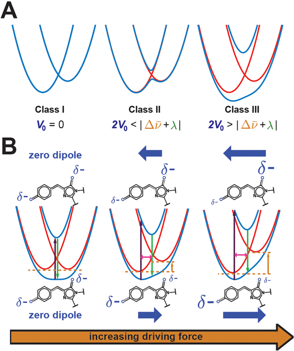
Evolution of potential energy curves with varying parameters. (A) Robin–Day classification scheme that separates mixed-valence compounds by the strength of the electronic coupling V₀. Blue and red depict the diabatic and adiabatic curves, respectively, showing that class II systems have a double-well potential in the ground state, while class III systems have a single well. (B) Influence of the driving force on the potential energy curves of the anionic GFP chromophore. As the driving force (orange arrow) increases, the absorption maximum (dark purple arrow) blue-shifts, the Stokes shift (difference between dark purple and green arrows) increases, the vibronic coupling (magenta arrow) increases, and the negative charge (size of δ−) is more localized, leading to a larger Stark tuning rate. The directions and magnitudes of the excited- and ground-state dipoles in each case are shown above and below the potential energy curves, respectively, as blue thick arrows. Note that, for the case on the left, while the schematic implies no dipole change upon excitation, the actual molecule may have a small nonzero dipole.