Classification of CT Scan Images of Lungs Using Deep Convolutional Neural Network with External Shape-Based Features

Abstract

In this paper, a simplified yet efficient architecture of a deep convolutional neural network is presented for lung image classification. The images used for classification are computed tomography (CT) scan images obtained from two scientifically used databases available publicly. Six external shape-based features, viz. solidity, circularity, discrete Fourier transform of radial length (RL) function, histogram of oriented gradient (HOG), moment, and histogram of active contour image, have also been identified and embedded into the proposed convolutional neural network. The performance is measured in terms of average recall and average precision values and compared with six similar methods for biomedical image classification. The average precision obtained for the proposed system is found to be 95.26% and the average recall value is found to be 69.56% in average for the two databases.

Introduction

Biomedical image processing plays a vital role in early identification of a disease and thereby preventing the extent of damage that can be caused by a disease in patients [1–3]. A comparison of various automation techniques for the classification of CT images of lung scans is given in [4]. Shape-based features have been widely used as constant feature markers for identifying the diseased area in a biomedical image; for instance, authors in [5] used two shape-based features—one based on lung-silhouette curvature and second based on minimal-polyline approximation for classification of images having emphysema using feedforward neural network. Lung-silhouette was captured by a contour drawn on the basis of cubic splines. Li et al. [6] proffered a shape-based visual saliency mechanism for extraction of lung regions in chest radiographs. Here, the X-ray image is first segmented into sub-regions using a graph segmentation approach and cubic spline interpolation method has been used to enhance these segmented regions. A salient value of each sub-region is extracted and the lung region is estimated by comparing these salient values. Abbasi et al. [7] also used a local shape-based feature set called curvature scale space and combined it with global features like eccentricity and circularity of an object shape-based approach to retrieve similar images. Further in [8], authors have proposed ROI-based approach for detection of breast cancer in the bio-medical images. Four feature vectors based on the shape are extracted, viz. solidity, circularity, discrete Fourier transform of radial length (RL) function, and histogram of Gaussian (HOG), and classification is achieved by using SVM classifier. Another ROI-based breast cancer detection method has been proposed by Wang et al. [9] where the input image database consists of a number of positive ROIs and normal ROIs. To check the performance of the system, various similarity thresholds have been used to measure the similarity between the queried ROI and extracted ROIs and those extracted ROIs with similarity more than threshold value have been used for classification purpose. Other image retrieval techniques that use texture-based features instead of shape-based features are summarized in [10–13].

In recent times, the concept of deep learning using convolutional neural network (CNN) is becoming popular for classification of bio-medical images. For instance, authors in [14] created a CNN having five convolutional layers, five max-pooling layers, two normalization layers, one fully connected and one softmax layer for classification of tumor in brain MR images. Authors in [15] presented a Caffe CNN framework for high-resolution CT (HRCT) images of lungs. They classified biomedical images using CNN architecture with two convolutional layers followed by a max-pooling layer. The output of this max-pooling layer is fed into a feedforward neural network architecture for final classification. Chung et al. [16] proposed a CNN by combining two Res-Net-50 CNNs. In each Res-Net-50 CNN, pre-trained weights of another CNN named as Image-Net over the same database are used. This CNN thereby formed is referred to as Siamese deep network and is used for classification of diabetic retinopathy images. Authors in [17] proposed a CNN with 25 convolutional layers, two fully connected layers, and one output layer for classification of datasets with medical images of brain MRI, breast MRI, and cardiac computed tomography angiogram (CTA). Here, a single CNN is proposed for three different types of medical images and it is shown that its performance is comparable to CNNs trained for a specific dataset. In [18], authors suggested a deep network with four convolutional and three pooling layers. The input consisted of 1553 axial, sagittal, and coronal views of pulmonary segment for classification of emphysema. The results have been compared with other complex CNN architectures and the proposed one has been claimed to be more suitable. Another CNN-based image retrieval system for lung images was proposed by authors in [19] in which the extracted features are encoded using fisher vector encoding and dimensionality reduction is done using principal component analysis (PCA). It is then fed into a multivariate regression model for classification. Campo et al. [20] proffered an approach based to detect the emphysema from X-ray images using a CNN with four convolutional layers, two max-pooling layers, two dense layers, one dropout, one flatter, and one output layer. An accuracy of 90.33% is achieved in this case.

Moreover, there are a number of medical image classification methods which use CNNs along with externally extracted features. For example, authors in [21] used a classification model where many texture-based features like local binary patterns and local ternary patterns are extracted from the images and then fed into three parallel CNNs at the same time. The output feature set is an input to SVM for final classification of images. In [22], a dynamic threshold-based local mesh ternary pattern (LMeTerP) is computed. The features extracted using this dynamic LMeTerP are then combined with CNN architecture to retrieve similar biomedical images. In [23], a dataset of 1500 medical images from different body parts like lung, brain, and heart is collected and downsampled. A patch-based feature set is then extracted using various filters and subsequently a parametric rectified linear unit is applied as an activation function. Finally, a deep convolutional network is applied to the feature set obtained and reconstruction of the images is achieved by minimizing the loss between predicted output image and obtained high-resolution image. Authors in [24] used a stochastic Hopfield network for detecting lung nodules in CT scan images. The features extracted using RBM are fed into a CNN with two convolutional layers, two sub-sampling layers, and one fully connected layer for final classification. The approach was classified between the benign and malignant nature of lung nodules.

It has also been observed in literature [21–24] that when a suitable CNN architecture is supported with external features, its performance is increased. Therefore, in this paper, a CNN architecture for medical image classification is proposed and its performance is analyzed with respect to other CNN-based medical image classification systems to prove its worthiness. Moreover, six external feature sets (four existing and two suggested) have also been introduced and when the proposed CNN-based system is combined with these six feature sets, its precision and recall are further increased by nearly 10.07% and 6.21% respectively. The paper is divided into following sections. “Background” explains the background of the various CNNs. The proposed CNN architecture followed by details of extracted features is given in “Proposed Work.” Experimental results are given in “Results and Discussions” and the paper is concluded in “Conclusion.”

Background

Basics of CNN

Convolutional neural networks are a specialized form of artificial neural networks with more number of hidden layers and advanced transfer functions (https://leonardoaraujosantos.gitbooks.io/artificial-inteligence/content/residual\_net.html). A simplest CNN architecture can have six layers as shown in Fig. 1.

1. Input layer: It holds the raw input image to be fed into convolutional layer.

2. Convolutional layer: It extracts the features from a given image by convoluting the kernel over the image. Here, hyper-parameters like stride (number of pixels the kernel can skip while convolution) can be tuned.

3. ReLU (rectified linear unit) layer: A ReLU layer performs a threshold operation to the input, and any value in the input less than zero is set to zero. Instead of making it as a separate layer, we can also embed it in the transfer function of the convolutional layer.

4. Pooling layer: It reduces the dimensions of feature maps as extracted by convolutional layer and thereby prevents overfitting.

5. Dense layer: Feature maps are flattened to create feature vector in this layer, which can then be fed into the final classification layer.

6. Classification layer: It predicts the class of the input image. Here, the number of neurons is same as the number of classes in the final output.

Fig. 1.

Architecture of a convolutional neural network

Parameters like number of convolutional layers, size of filters, number of max-pooling layers, size of stride, number of hidden neurons in dense layer, and transfer function are considered as training parameters for a given CNN.

ImageNet-VGG-f Architecture

It is one of the popular CNN architectures explored in [21] for medical image classification with remarkable performance. Its original architecture is suggested by authors in [25, 26] in which there are five convolutional layers, three max-pooling layers, two dense layers, and one output layer. In [21], the performance of ImageNet-VGG-f architecture is claimed to be the one of the best over other ImageNet architectures for a medical image dataset.

In this paper, the architecture of ImageNet-VGG-f CNN has been modified as explained in the next section by scraping the convolutional layer and incorporating externally extracted feature vectors.

Proposed Work

Proposed CNN Architecture

Many CNN architectures have been proposed by authors in the past, like in [24, 27] for classification of CT scan images of lungs. One such architecture is an ImageNet-VGG-f feature-based CNN model which has been proposed by authors in [21]. In this paper, a simplest modified version of ImageNet-VGG-f CNN with lesser number of layers has been proposed. Moreover, six external features (four existing and two proposed) as described in “Extracted Features” have also been suggested and the combined performance of these features with proposed CNN is evaluated. As discussed in “Basics of CNN,” since the role of convolutional layer is to extract features from the input image, this layer is dropped in the proposed CNN architecture due to the externally extracted features given as an input to it. Thereby, this architecture is comprised of one ReLU layer, one max-pooling layer, one dense layer, and finally one classification layer as shown in Fig. 2. The stride is set to 1 and also the pool size is set to 1 × 1 for maximum precision and recall as discussed in (https://in.mathworks.com/help/nnet/examples/create-simple-deep-learning-network-for-classification.html).

Fig. 2.

Proposed CNN architecture

Further, the architecture is tested on different numbers of epochs and the maximum precision and recall values are obtained when the CNN model is trained with 200 epochs. To verify if the architecture is best suited for classification, we extended the architecture and added more number of max-pooling layers and dense layers. It has been observed that there is no improvement in the performance of the system. Therefore, saturation in performance has been observed for the proposed CNN architecture.

Extracted Features

A contour is first extracted from an input image as given in “Contour Extraction.” This contour is further used for extraction of external features as explained in subsequent subsections.

Contour Extraction

The input image is first segmented into a foreground (object) and a background region using active contour method. For extracting the active contour, curves in the image are specified to find the boundary of foreground object [28]. These curves are evolved iteratively to detect objects in the image I. This method of contour extraction is also referred as the snake model for contour extraction. The biomedical images used for analysis of our proposed feature set are 8-bit grayscale images. If C(s) is a parameterized curve defined on an image, C′(s) is its first derivative and C″(s) is its second derivative, then the snake model is described by inf(J₁(C)) [28]. Here, inf(J₁(C)) represents a minimization problem for J₁(C) where J₁(C) is described in Eq. (1), in which α, β, and λ are positive parameters.

$$J_1\left(C\right)=\alpha {\int }_0^1{\left|C^{\prime }\left(s\right)\right|}^2\mathrm{ds}+\beta {\int }_0^1\mid C^{\prime \prime }\left(s\right)\mid \mathrm{ds}-\lambda {\int }_0^1{\left|△I\left(C\left(s\right)\right)\right|}^2\mathrm{ds}$$ 1

The first two parameters control the smoothness of the contour and the third parameter takes the contour towards object in the image. We reiterate this process to obtain more points for defining the points on the active contour. For the proposed algorithm, number of iterations used was 10 as beyond 10, no new points were adding to the given contour.

External Features

From the contour obtained in the previous section, six features are extracted. Out of these six features, four features, viz. solidity, circularity, discrete Fourier transformation (DFT) of radial length (RL) function, and histogram of oriented gradients (HOG) are the same as in [8] whereas two additional features are histogram and second-order moments of the image. These additional features have been added to further improve the performance of the system. If there are n points on the active contour represented as x_i and y_i where i = 1…n, then we can define the feature vectors in the following way:

1. Solidity: It represents the relationship between the areas enclosed by the active contour with respect to the area enclosed by the convex hull of the active contour. It is calculated using Eq. (2).

$$\mathit{\text{Solidity}}=\frac{A}{H}$$ 2

where A and H denote the area enclosed by the active contour and its corresponding convex hull respectively and both parameters are calculated using Eq. (3).

$$A=\frac{1}{2}{\sum }_{i=1}^{n-1}\left(x_{i+1}-x_i\right)\left(y_{i+1}-y_i\right)$$ 3

• (b)Circularity (F_circ): It calculates the extent of circular nature of the extracted contour and can be calculated using Eq. (4).

$$F_{\text{circ}}=1-\left(4\pi A/P^2\right)$$ 4

where P is the perimeter of the closed contour which can be calculated using Eq. (5) and A represents contour area as given in Eq. (3).

$$P=\sum _{i=1}^{n-2}\sqrt{\left(x_{i+1}-x_i\right)+\left(y_{i+1}-y_i\right)}$$ 5

• (c)DFT coefficients of the RL function:

The RL function is defined in Eq. (6). Radial length is the distance of points in the contour from the centroids of the contour. If x_c and y_c are coordinates of contour centroid, then radial length RL(i) of the ith point (x_i, y_i) is given as:

$$\mathrm{RL}\left(i\right)=\sqrt{{\left(x_i-x_c\right)}^2+{\left(y_i-y_c\right)}^2}$$ 6

We calculate n DFT values of the above function using Eq. (7).

$$\mathrm{DFT}\_\mathrm{RL}\left(u\right)=\frac{1}{n}{\sum }_{i=0}^n\mathrm{RL}\left(i\right).e^{\frac{-j2\mathit{\pi ui}}{n}}$$ 7

where u = 1…n.

• (d)HOG: It calculates the distribution of gradients for an image I. In the first step, the gradient magnitude |I′| and orientation argI′ is calculated by using Eqs. (8) and (9) for each pixel location (i, j) [8].

$$\mid I’\left(i,j\right)\mid =\sqrt{I_x{\left(i,j\right)}^2+I_y{\left(i,j\right)}^2}$$ 8

$$argI’\left(i,j\right)=arctan\frac{I_y\left(i,j\right)}{I_x\left(i,j\right)}$$ 9

where I_x and I_y represent x and y components of gradient image of I.

$$I_x\left(i,j\right)=I\left(i+1,j\right)-I\left(i,j\right)$$ 10

$$I_y\left(i,j\right)=I\left(i,j+1\right)-I\left(i,j\right)$$ 11

Further, the image is divided into various blocks of 16 × 16 pixels. Each block is comprised of 2 × 2 cells where each cell is made up of 8 × 8 pixels. Thus, the blocks are 1 cell distant horizontally. We thereby calculate the histogram of each cell and then concatenate the four cell histograms in each block to form a single block histogram feature bl. This block feature is then normalized using Eq. (12).

$$\mathit{bl}\leftarrow \frac{\mathit{bl}}{\sqrt{{\left|\left|\mathit{bl}\right|\right|}^2+\epsilon }}$$ 12

Here, ε is a small positive constant that prevents divide by zero error. Finally, the normalized block histograms are concatenated to form the final feature vector.

• (e)Histogram of the image having active contour.

Histogram of an image represents the number of pixel intensities that lies in a bin. A 256 equally spaced bin histogram is created for the segmented image having active contours. This 256 × 1 vector is then used as a feature vector.

• (f)Moment of the image having contour.

Central moment best describes the information related to the shape of an image (http://www.csie.ntnu.edu.tw/~bbailey/Moments\%20in\%20IP.html). Thereby, central moment of the image having active contour is used as another feature vector. The order is kept as 2 since it provides contrast information within the image and higher order moments are difficult to compute (http://www.csie.ntnu.edu.tw/~bbailey/Moments\%20in\%20IP.html). For a 2D image of dimension M × N, moment can be calculated by using Eq. (13).

$$\text{Moment}={\sum }_{x=0}^{256}{\left(x-m\right)}^{2}p\left(x\right)$$ 13

where x is gray scale value and p(x) is its probability of occurrence in the image. Here, m represents average intensity of the image and is defined as

$$m={\sum }_{x=0}^{256}x.p\left(x\right)$$ 14

All these features are then fed as input to CNNs described in “Proposed CNN Architecture” for classification and their performance is compared. Also Fig. 3 gives a schematic representation of the steps in the proposed work.

Fig. 3.

Schematic representation of the proposed scheme for classification

Results and Discussions

Two datasets having CT scan images of lungs (http://image.diku.dk/emphysema_database/, http://www.via.cornell.edu/lungdb.html) profoundly used by the research community have been used. These datasets comprised of 124 and 100 samples from different patients as summarized in Table 1. The results are obtained on a computational device with 8-GB RAM and 2.0 GHz frequency. MATLAB is used for simulation purpose.

Table 1.

Details of the database used

Database no.	No. of slices	Resolution of images	Tube voltage (kV)	Format
1	124	512 × 512	120	.tiff
2	180	512 × 512	120	.dcm

The first dataset is comprised of CT scan images of around 39 subjects (9 never-smokers, 10 smokers, and 20 smokers with chronic obstructive pulmonary disease (COPD or emphysema)) (http://image.diku.dk/emphysema_database/). There are 124 slices obtained from top, middle, and lower view of lungs. All images are divided into four groups for classification—normal tissue (NT), centrilobular emphysema (CLE), paraseptal emphysema (PSE), and pan-lobular emphysema (PLE).

The second dataset is obtained from ELCAP lung database. Out of the four repositories available in (http://www.via.cornell.edu/lungdb.html), we selected W0011-W0020 repository. It had CT scan images for 10 different groups and image classification will be done for these 10 groups. Each slice is of 1.25 mm thickness and is obtained in a single breath hold using CT scan. The dataset is also provided with the location of nodules in the lungs of the patient. The details of these two datasets are given in Table 2. Images of patients from four different groups of dataset 1 and 10 different groups of dataset 2 are given in Figs. 4 and 5 respectively.

Table 2.

Parameters for different architectures

Parameters	Best [29]	Google-Arch	MLC-CNN [19]	ImageNet-VGG-f	Base approach with CNN	Proposed CNN architecture
No. of convolutional layers	13	2	5	5	–	–
No. of inception layers	–	9	–	–	–	–
No. of max-pooling layers	5	2	–	3	1	1
Pool size for pool1 and pool2	2 × 2	1 × 1	–	1 × 1	1 × 1	1 × 1
Stride for pool1 and pool2	1	1	–	1	1	1
No. of ReLU layers	–	–	–	–	1	1
No. of dense layers	3	1	2	2	1	1
No. of classification layers	1	1	1	1	1	1
Number of epochs used for training	200	200	200	200	200	200

Fig. 4.

CT images of patients with emphysema condition as a minimal or no emphysema, b centrilobular emphysema, c paraseptal emphysema, and d pan-lobular emphysema

Fig. 5.

Images obtained from ELCAP lung database for 10 different groups

Figure 6a shows an original image from database 1 from which active contour region is extracted and accordingly Fig. 6b, c shows the contour generation when Eq. (1) is applied once and then 10 times respectively. Similarly, Fig. 7 shows the sample image and its contour generation from database 2.

Fig. 6.

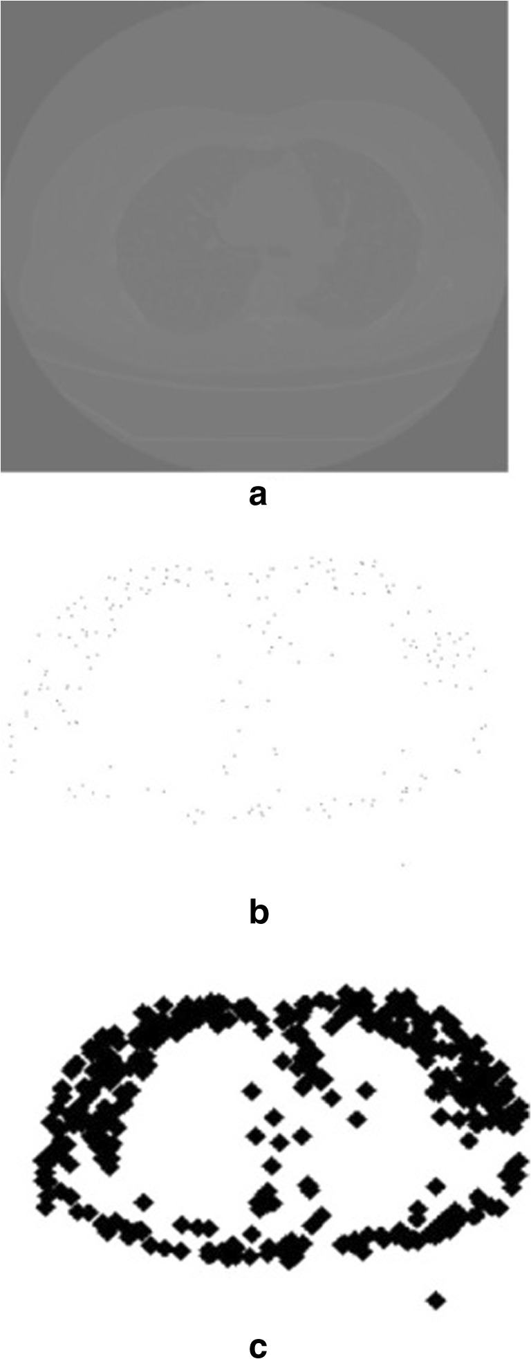
a Sample image (database 1). b Active contour extracted after Eq. (1) applied once. c Contour extracted after Eq. (1) applied 10 times

Fig. 7.

a Sample image (database 2). b Active contour extracted after Eq. (1) applied once. c Contour extracted after Eq. (1) applied 10 times

From these active contours, six feature vectors have been computed as described in “Proposed Work.” These feature vectors are then fed into proposed CNNs for the classification of images of different groups. The parameters for different CNNs used in the experimental results are summarized in Table 2.

Thereafter, the recall and precision are calculated for each group. The results of different algorithms are compared based on the average retrieval precision (ARP) and average retrieval rate (ARR) respectively. It can be calculated using Eqs. (15) and (17).

$$\mathrm{ARP}=\frac{{\sum }_{i=0}^{\mathrm{w}}P\left(i\right)}{w}$$ 15

for q ≤ 10

$$P\left(i\right)=\frac{\text{number of relevant images retrieved of}\mathrm{a}\text{group}}{\text{total number of images retrieved for that group}}$$ 16

Further, w is the number of images in the database and q is the number of similar images retrieved from the database. Similarly,

$$\mathrm{ARR}=\frac{{\sum }_{i=0}^{w}R\left(i\right)}{w}$$ 17

for q ≥ 10where R(i) denotes the recall value and is defined as

$$R\left(i\right)=\frac{\text{number of relevant images retrieved of}\mathrm{a}\text{group}}{\text{total number of relevant images in the database for that group}}$$ 18

A detailed comparison of recall and precision values obtained for the various algorithms are summarized in Tables 3, 4, 5, and 6. Tables 3 and 5 compare various algorithms for recall values in the case of database 1 and database 2 respectively whereas Tables 4 and 6 compare precision for various algorithms in the case of databases 1 and 2 respectively. Each precision and recall value corresponds to one particular group of the database.

Table 3.

Recall values for database 1

	Best [29]	Google-Net CNN [27]	MLC-CNN [19]	ImageNet-VGG-f CNN architecture [21]	[8]	Base approach [8] with proposed CNN	Prop. features with proposed architecture
Group 1	70.43	51.10	66.20	70.80	62.40	70.30	75.90
Group 2	59.30	56.20	60.22	72.30	59.80	75.90	76.30
Group 3	61.12	52.40	67.30	65.40	60.30	72.40	74.80
Group 4	60.77	51.50	66.60	69.20	58.90	73.40	76.10
Avg. RR	62.90	52.80	65.08	69.42	60.35	73.00	75.77

Table 4.

Precision values for database 1

	Best [29]	Google-Net CNN [27]	MLC-CNN [19]	ImageNet-VGG-f CNN architecture [21]	[8]	Base approach [8] with proposed CNN	Prop. features with proposed architecture
Group 1	63.40	50.00	76.70	78.90	70.50	75.67	92.19
Group 2	85.70	70.40	86.10	89.70	75.80	84.40	92.80
Group 3	83.10	79.80	84.20	94.10	74.30	86.50	93.10
Group 4	88.10	84.40	88.30	86.10	72.10	81.10	91.10
Avg. RP	80.07	71.15	83.82	87.20	73.17	81.91	92.29

Table 5.

Recall values for database 2

	Best [29]	Google-Net CNN [27]	MLC-CNN [19]	ImageNet-VGG-f CNN architecture [21]	[8]	Base approach [8] with proposed CNN	Prop. features with proposed architecture
Group 1	40.33	51.30	45.00	52.40	41.80	42.10	55.90
Group 2	41.22	42.30	48.10	48.90	45.30	46.70	52.30
Group 3	43.67	41.20	57.70	60.30	50.60	44.20	61.30
Group 4	60.55	57.10	58.90	58.90	52.70	56.90	60.70
Group 5	46.45	42.40	42.30	48.90	43.10	43.20	53.40
Group 6	55.86	48.80	54.87	57.80	52.10	52.10	59.80
Group 7	51.89	45.70	50.70	54.30	49.60	47.80	58.90
Group 8	88.92	72.30	90.40	89.70	87.30	82.30	94.30
Group 9	48.23	46.70	52.30	57.70	47.90	47.80	56.70
Group 10	73.10	72.30	75.80	72.50	72.10	74.30	80.70
Avg. RR	55.02	52.01	57.60	60.14	54.25	53.74	63.40

Table 6.

Precision values for database 2

	Best [29]	Google-Net CNN [27]	MLC-CNN [19]	ImageNet-VGG-f CNN architecture [21]	[8]	Base approach [8] with proposed CNN	Prop. features with proposed architecture
Group 1	86.10	91.10	100.00	98.70	73.40	84.50	100.00
Group 2	90.22	87.50	92.80	96.70	74.10	86.30	95.50
Group 3	86.80	86.70	90.40	97.50	72.30	87.80	98.70
Group 4	90.20	87.90	92.90	85.60	71.10	90.90	98.50
Group 5	90.60	91.40	94.44	93.30	75.40	97.60	99.10
Group 6	93.20	88.90	90.80	92.50	78.90	89.90	96.10
Group 7	95.89	91.30	92.00	95.60	73.90	84.80	97.80
Group 8	98.80	93.40	92.50	97.70	72.90	87.60	99.30
Group 9	96.54	95.90	97.80	92.30	79.90	85.50	98.70
Group 10	98.22	96.90	98.40	96.50	75.80	89.90	98.60
Avg. RP	92.65	91.10	94.20	94.64	74.77	88.48	98.23

It can be seen from these tables that the proposed CNN-based system when supported with suggested external features consistently outperforms all remaining techniques. For database 1, as shown in Table 3, it produces 6.35% more recall value than original ImageNet-VGG-f architecture [21] whereas it is larger by 2.77% when the proposed CNN architecture is combined with existing four features which are suggested in [8]. Similarly in Table 4, the average recall value for the proposed system is greater by 3.26% than the CNN architecture of [21]. In terms of precision, for database 1, proposed system returns approximately 5% and 10% more values than that of [21] and proposed CNN with four existing features. However, for database 2, proposed system is better by 3.59% and 9.75% when compared with the same methods. Further, it can be seen that the retrieval system suggested in [21] remains the second best performer in terms of ARP for both databases.

Conclusion

The proposed work is a simplified and less complex form of ImageNet-VGG-f CNN architecture for classification of CT images of lungs. In this work, two additional external features over those suggested in [10] have also been introduced and total six external features have been incorporated in the proposed CNN model. The performance of the proposed system is compared with other six parallel approaches to justify its superiority using two scientifically used databases. The proposed system shows an improvement of 4.34% in terms of ARP and 4.78% in terms of ARR in average for both databases over ImageNet-VGG-f CNN architecture.

References

- 1.Siegel RL, Miller KD, Jemal A. Cancer statistics, 2016. CA: a cancer journal for clinicians. 2016;66(1):7–30. doi: 10.3322/caac.21332. [DOI] [PubMed] [Google Scholar]
- 2.De Azevedo-Marques, Paulo Mazzoncini, Arianna Mencattini, Marcello Salmeri, and Rangaraj M. Rangayyan, eds. "Medical Image Analysis and Informatics: Computer-Aided Diagnosis and Therapy.", CRC Press, Taylor and Francis, 2017.
- 3.Purwar RK, Srivastava V. Recent advancements in detection of cancer using various soft computing techniques for MR images, in Progress of Advanced Computing and Intelligent Engineering. Singapore: Springer; 2018. pp. 99–108. [Google Scholar]
- 4.Sluimer I, Schilham A, Prokop M, Van Ginneken B. Computer analysis of computed tomography scans of the lung: A survey. IEEE transactions on medical imaging. 2006;25(4):385–405. doi: 10.1109/TMI.2005.862753. [DOI] [PubMed] [Google Scholar]
- 5.Coppini G, Miniati M, Paterni M, Monti S, Ferdeghini EM. Computer-aided diagnosis of emphysema in COPD patients: Neural-network-based analysis of lung shape in digital chest radiographs. Medical engineering and physics. 2007;29(1):76–86. doi: 10.1016/j.medengphy.2006.02.001. [DOI] [PubMed] [Google Scholar]
- 6.Li, Xin, Leiting Chen, and Junyu Chen, "A visual saliency-based method for automatic lung regions extraction in chest radiographs.", In 14th International Computer Conference on Wavelet Active Media Technology and Information Processing (ICCWAMTIP), pp. 162-165. IEEE, 2017.
- 7.Abbasi S, Mokhtarian F, Kittler J. Curvature scale space image in shape similarity retrieval. Multimedia systems. 1999;7(6):467–476. doi: 10.1007/s005300050147. [DOI] [Google Scholar]
- 8.Tsochatzidis L, Zagoris K, Arikidis N, Karahaliou A, Costaridou L, Pratikakis I. Computer-aided diagnosis of mammographic masses based on a supervised content-based image retrieval approach. Pattern Recognition. 2017;71:106–117. doi: 10.1016/j.patcog.2017.05.023. [DOI] [Google Scholar]
- 9.Wang XH, Park SC, Zheng B. Assessment of performance and reliability of computer-aided detection scheme using content-based image retrieval approach and limited reference database. Journal of digital imaging. 2011;24(2):352–359. doi: 10.1007/s10278-010-9281-x. [DOI] [PMC free article] [PubMed] [Google Scholar]
- 10.Park, Yang Shin, Joon Beom Seo, Namkug Kim, Eun Jin Chae, Yeon Mok Oh, Sang Do Lee, Youngjoo Lee, and Suk-Ho Kang, "Texture-based quantification of pulmonary emphysema on high-resolution computed tomography: comparison with density-based quantification and correlation with pulmonary function test.", Investigative radiology, 43(6), 395-402, 2008. [DOI] [PubMed]
- 11.Nanni L, Lumini A, Brahnam S. Local binary patterns variants as texture descriptors for medical image analysis. Artificial intelligence in medicine. 2010;49(2):117–125. doi: 10.1016/j.artmed.2010.02.006. [DOI] [PubMed] [Google Scholar]
- 12.Moura DC, Guevara López MA. An evaluation of image descriptors combined with clinical data for breast cancer diagnosis. International journal of computer assisted radiology and surgery. 2013;8(4):561–574. doi: 10.1007/s11548-013-0838-2. [DOI] [PubMed] [Google Scholar]
- 13.Srivastava V, Purwar R. An extension of local mesh peak valley edge based feature descriptor for image retrieval in bio-medical images. ADCAIJ: Advances in Distributed Computing and Artificial Intelligence Journal. 2018;7(1):77–89. doi: 10.14201/ADCAIJ2018717789. [DOI] [Google Scholar]
- 14.Pang S, Yu Z, Orgun MA. A novel end-to-end classifier using domain transferred deep convolutional neural networks for biomedical images. Computer methods and programs in biomedicine. 2017;140:283–293. doi: 10.1016/j.cmpb.2016.12.019. [DOI] [PubMed] [Google Scholar]
- 15.Karabulut, Esra Mahsereci, and Turgay Ibrikci. "Emphysema discrimination from raw HRCT images by convolutional neural networks." In 9th International Conference on Electrical and Electronics Engineering (ELECO), pp. 705-708, IEEE, 2015.
- 16.Chung, Y. A., and Weng, W. H., "Learning deep representations of medical images using Siamese CNNs with application to content-based image retrieval", Computer Vision and Pattern Recognition, Cornell University, arXiv:1711.08490, 2017.
- 17.Moeskops P, Wolterink JM, van der Velden BH, Gilhuijs KG, Leiner T, Viergever MA, Išgum I. Deep learning for multi-task medical image segmentation in multiple modalities. In International Conference on Medical Image Computing and Computer-Assisted Intervention. Cham: Springer; 2016. pp. 478–486. [Google Scholar]
- 18.Bermejo-Peláez, David, Raúl San José Estepar, and María J. Ledesma-Carbayo. "Emphysema classification using a multi-view convolutional network.", In 15th International Symposium on Biomedical Imaging (ISBI 2018), pp. 519-522. IEEE, 2018. [DOI] [PMC free article] [PubMed]
- 19.Gao, M., Xu, Z., Lu, L., Harrison, A. P., Summers, R. M., and Mollura, D. J., "Holistic interstitial lung disease detection using deep convolutional neural networks: Multi-label learning and unordered pooling", Computer Vision and Pattern Recognition, Cornell University, arXiv:1701.05616, 2017.
- 20.Campo, Mónica Iturrioz, Javier Pascau, and Raúl San José Estépar. "Emphysema quantification on simulated X-rays through deep learning techniques." In 2018 IEEE 15th International Symposium on Biomedical Imaging (ISBI 2018), pp. 273-276. IEEE, 2018. [DOI] [PMC free article] [PubMed]
- 21.Nanni L, Ghidoni S, Brahnam S. Handcrafted vs. non-handcrafted features for computer vision classification. Pattern Recognition. 2017;71:158–172. doi: 10.1016/j.patcog.2017.05.025. [DOI] [Google Scholar]
- 22.Srivastava Varun, Purwar RK, Jain Anchal, "A dynamic threshold-based local mesh ternary pattern technique for biomedical image retrieval. International Journal of Imaging Systems and Technology, Vol. 29(2), pp: 168-179, 2018.
- 23.Liu H, Xu J, Wu Y, Guo Q, Ibragimov B, Xing L. Learning deconvolutional deep neural network for high resolution medical image reconstruction. Information Sciences. 2018;468:142–154. doi: 10.1016/j.ins.2018.08.022. [DOI] [Google Scholar]
- 24.Hua, Kai-Lung, Che-Hao Hsu, Shintami Chusnul Hidayati, Wen-Huang Cheng, and Yu-Jen Chen. "Computer-aided classification of lung nodules on computed tomography images via deep learning technique.", OncoTargets and therapy 8, 2015. [DOI] [PMC free article] [PubMed]
- 25.Simonyan, Karen, and Andrew Zisserman, "Very deep convolutional networks for large-scale image recognition", Computer Vision and Pattern Recognition, Cornell University, arXiv: 1409.1556, 2014.
- 26.Wozniak P, Afrisal H, Esparza RG, Kwolek B. International Conference on Computer Vision and Graphics. Cham: Springer; 2018. Scene recognition for indoor localization of mobile robots using deep CNN; pp. 137–147. [Google Scholar]
- 27.Hoo-Chang S, Roth HR, Gao M, et al. Deep convolutional neural networks for computer-aided detection: CNN architectures, dataset characteristics and transfer learning. IEEE transactions on medical imaging. 2016;35(5):1285–1298. doi: 10.1109/TMI.2016.2528162. [DOI] [PMC free article] [PubMed] [Google Scholar]
- 28.Chan TF, Sandberg BY, Vese LA. Active contours without edges for vector-valued images. Journal of Visual Communication and Image Representation. 2000;11(2):130–141. doi: 10.1006/jvci.1999.0442. [DOI] [Google Scholar]
- 29.Nanni L, Paci M, Brahnam S, Ghidoni S. An ensemble of visual features for Gaussians of local descriptors and non-binary coding for texture descriptors. Expert Systems with Applications. 2017;82:27–39. doi: 10.1016/j.eswa.2017.03.065. [DOI] [Google Scholar]