. 2020 Mar 11;9:e53672. doi: 10.7554/eLife.53672

Figure 2. Flagellar filament purified from wild-type L. biflexa Patoc with asymmetric sheath layer visualized by cryo-tomographic sub-tomogram averaging.

(A) Cryo-tomographic slice of the flagellar filament in vitrified ice. Dashed box denotes the approximate dimensions extracted for sub-tomographic averaging. (B) Final averaged volume (isosurface representation) of the flagellar filament denoting segmented regions of sheath (red, green, and blue) and core (yellow). The red sheath regions are located on the inner curvature or ‘concave’ side of the filament, whereas the blue and green sheath regions are located on the outer curvature, or ‘convex’ side. (C) Cross-sectional view of the sub-tomographic average; the filament diameter ranges from 210 to 230 Å. (D – E) Rotated views of the sub-tomographic average. (F, G) Wild-type map axial and lateral cross-sections (respectively), highlighting asymmetric features including the ‘groove’ on the filament inner curvature. The white dashed line in (F) indicates the geometry of the lateral density cross-section in panel (G). (H) Projected wild-type map cross-section, filtered to 18 Å resolution, showing features corresponding to core and sheath elements. (I) Projected fcpB map cross-section, highlighting differences with the wild-type projection in H. Four missing densities on the convex side (blue asterisks) correspond to fitted locations of FcpB in the wild-type map; an additional missing density on the concave side (red asterisk) is provisionally assigned as FlaA1 and/or FlaA2 (see text).

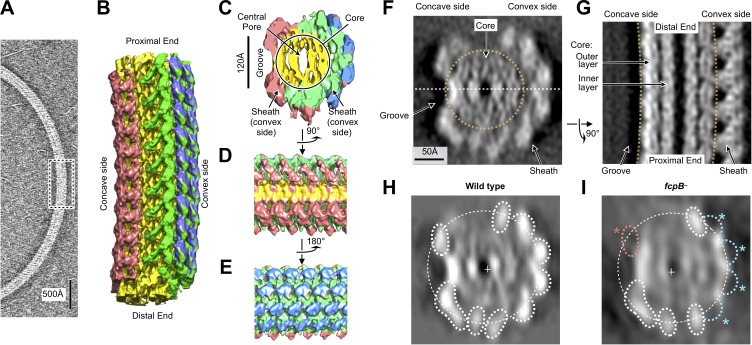
Figure 2.

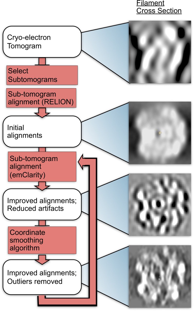
Figure 2—figure supplement 1. Methods flow chart.

Figure 2—figure supplement 1.

Cross-sections of subtomograms or subtomogram averages resulting from each step are shown on the right.
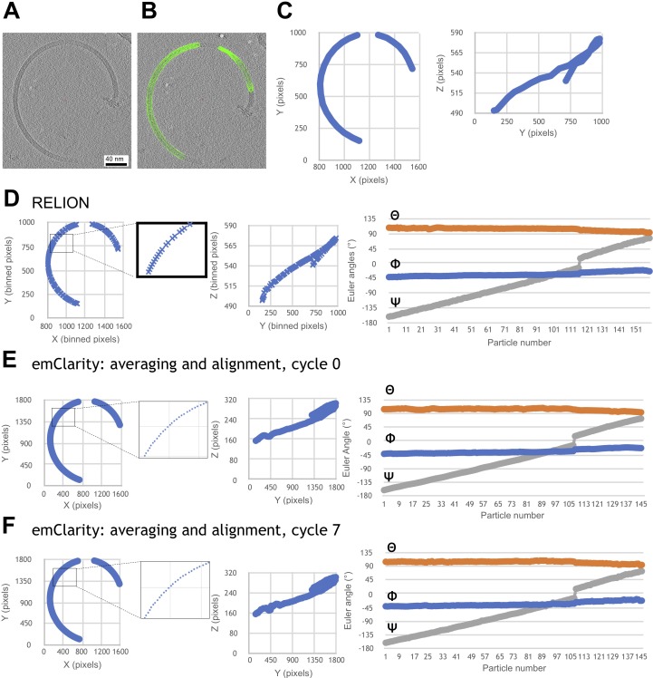
Figure 2—figure supplement 2. Progressive improvement of alignment parameters for a representative filament, after various stages of refinement.

Figure 2—figure supplement 2.

The refinement procedure incorporated an in-house smoothing algorithm that rectifies gaps, duplicates and outliers to obtain continuous 3D coordinate models of every subunit from each selected filament segment. (A) Section through a reconstructed tomogram of a purified L. biflexa wild-type flagellar filament. (B) Particle selection (green spheres) that selects the filament trajectory through the tomogram slice. (C) Particle X/Y (left) and Y/Z (right) coordinates selected in B. Tomograms and coordinates shown here correspond to a binning of 2, at 5.208 Å/pixel. (D) Filament trajectory (XYZ coordinates and Euler angles) following the initial RELION refinement step. (E) Filament trajectory output following the first cycle of emClarity refinement. Application of the smoothing algorithm after the RELION step eliminates gaps seen in some sections of the filament trace (compare insets in panels D and E). (F) Filament trajectory following an additional smoothing step, followed by a second pair of emClarity/smoothing steps.
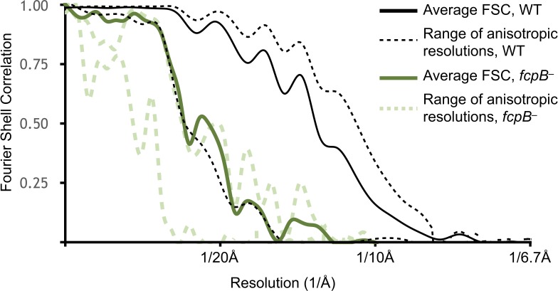
Figure 2—figure supplement 3. Resolution estimates for wild-type and fcpB subtomogram average reconstructions.

Figure 2—figure supplement 3.

Shown in dashed lines are Fourier shell correlation (FSC) curves that capture the resolution anisotropy using local sectors (‘cones’) in Fourier space. The corresponding resolution estimates range from ~9 Å in the best directions (perpendicular to the filament supercoiling axis, i.e. directions parallel to specimen ice layer plane) to ~18 Å in the worst direction (parallel to filament supercoiling axis, i.e. a vector perpendicular to the specimen ice layer plane). The latter direction corresponds to the ‘missing cone’ in our data due to a combination of strongly preferred filament orientation and limited tilt angle in the tomographic data collections. Resolution anisotropy results in a marked elongation of map features in this direction (orthogonal to the viewing plane in Figure 2A,B; vertical direction in Figure 2C–E). Results are only shown for the highest and lowest-resolution FSC cones.
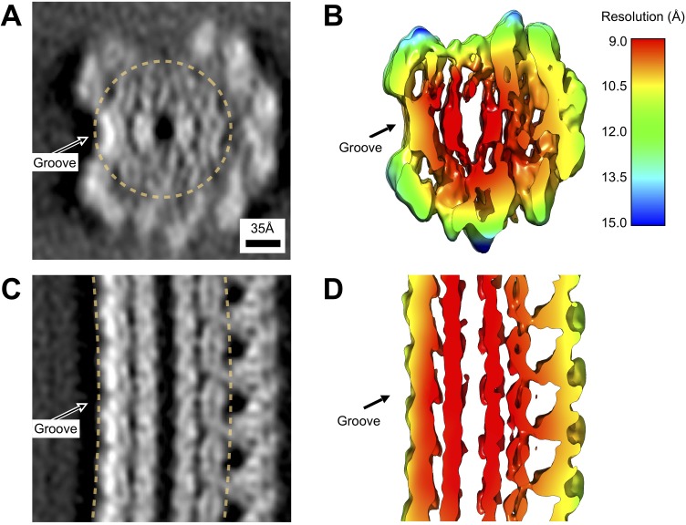
Figure 2—figure supplement 4. Local resolution estimates for the wild-type L. biflexa flagellar filament subtomogram average reconstruction.

Figure 2—figure supplement 4.

(A, C) Projected thin cross-sections of the subtomogram average, revealing the presence of nanometer-scale features. An arrow marks the groove, corresponding to a systematic absence of sheath density on one side of the filament. (B, D) Slices through the corresponding density isosurface, colored by estimated local resolution (see Materials and methods). The reported average resolution within the core ranges from 9 to 10 Å. Within the sheath, the reported resolution ranges from 10 to 13 Å, with excursions up to ~15 Å found at the top of the axial cross section (C).
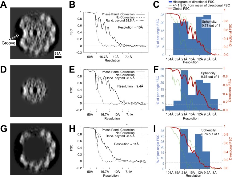
Figure 2—figure supplement 5. Directional resolution estimates for the wild-type Leptospira flagellar filament map, with separate estimates for masked core and sheath subregions.

Figure 2—figure supplement 5.

(A, D, G) Map cross-sections following application of the three masks used during these calculations, corresponding to the whole filament, core, and sheath regions, respectively (see Methods). (B, E, H) Non-directional Fourier Shell Correlation estimates for the three masked regions, calculated with the Relion software suite. (C, F, I) Directional Fourier Shell Correlation estimates for the three masked regions using the 3D FSC program (Tan et al., 2017) (see Materials and methods). The histogram (blue bars) reports the distribution of estimated resolutions for different angular directions (conical regions in Fourier space). Due to strongly preferred filament orientations in the sample (see Figure 1—figure supplement 1), a cone of data is missing from the map Fourier transform. As a result, a significant drop-off is observed in the reported resolution for angular directions that coincide with the missing cone, as reflected in the histogram: reported resolutions are distributed widely, from ~35 Å in the worst directions (those close to the vertical axis in (A, D, G) to ~8 Å in the best directions. Although this resolution anisotropy leads to ‘smearing’ of density features (vertical direction in panels (A), (D), (G), the asymmetric groove is large enough to be readily resolved in the wild-type map. While features on the left side in panels (A), (D), (G) (where the groove is located) diverge from the right side (where there is no groove), the average map resolution is comparable at these two locations (Figure 2—figure supplement 4), supporting the observed asymmetry between the two sides of the filament. See Figure 3—figure supplement 4.