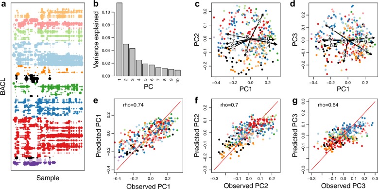
Fig. 4. Observed and predicted distributions of BACLs along principal axes of abundance variation.
a BACL abundance profiles (one BACL per line; the 99 most abundant BACL shown) across all 124 samples, with dot size proportional to log abundance in the sample, using the same color schema as in Fig. 3 but with additional taxa shown in black. b–d Principal coordinates analysis of BACL abundance profiles, with b displaying proportion of variation explained by the ten first principal coordinates (PC) and c, d plotting the BACLs along the first three principal coordinates. The arrows indicate relationships between the principal coordinates and measured environmental parameters (see Methods), where the numbers correspond to 1: salinity; 2: depth; 3: oxygen; 4: temperature; 5: filter size; 6: nitrate; 7: phosphate; 8: silicate; 9: chlorophyll a; 10: dissolved organic carbon. e–g Machine learning predicted (gradient boosting using gene profiles) vs. observed values of principal coordinate scores, with e displaying results for PC1, f for PC2 and g for PC3. Rho-values indicate Spearman rank correlation coefficients between predicted and observed values (all correlations P < 10-16). Prediction results for PC1–PC10 using different machine learning algorithms can be found in Supplementary Table 2.

