

Abstract
Reliably predicting in vivo efficacy from in vitro data would facilitate drug development by reducing animal usage and guiding drug dosing in human clinical trials. However, such prediction remains challenging. Here, we built a quantitative pharmacokinetic/pharmacodynamic (PK/PD) mathematical model capable of predicting in vivo efficacy in animal xenograft models of tumor growth while trained almost exclusively on in vitro cell culture data sets. We studied a chemical inhibitor of LSD1 (ORY‐1001), a lysine‐specific histone demethylase enzyme with epigenetic function, and drug‐induced regulation of target engagement, biomarker levels, and tumor cell growth across multiple doses administered in a pulsed and continuous fashion. A PK model of unbound plasma drug concentration was linked to the in vitro PD model, which enabled the prediction of in vivo tumor growth dynamics across a range of drug doses and regimens. Remarkably, only a change in a single parameter—the one controlling intrinsic cell/tumor growth in the absence of drug—was needed to scale the PD model from the in vitro to in vivo setting. These findings create a framework for using in vitro data to predict in vivo drug efficacy with clear benefits to reducing animal usage while enabling the collection of dense time course and dose response data in a highly controlled in vitro environment.
Study Highlights.
WHAT IS THE CURRENT KNOWLEDGE ON THE TOPIC?
☑ Mechanistic pharmacokinetic/pharmacodynamic (PK/PD) modeling enables multiscale (cell culture to in vivo) predictions of drug efficacy by accounting for system‐specific differences.
WHAT QUESTION DID THIS STUDY ADDRESS?
☑ How can we predict in vivo anticancer drug efficacy primarily from in vitro data sets?
WHAT DOES THIS STUDY ADD TO OUR KNOWLEDGE?
☑ We found in vivo tumor growth dynamics may be predicted from in vitro data when linking in vivo PK corrected for fraction unbound with a PK/PD model that quantitatively integrates knowledge and relationship among drug exposure, PD response, and cell growth inhibition collected solely from in vitro with pulse and continuous drug exposure. In addition, PD response is scaled to in vivo by accounting for the differences in tumor cell growth dynamics without drug. Although more cell lines and drugs should be tested, this study may suggest general applicability of this approach.
HOW MIGHT THIS CHANGE CLINICAL PHARMACOLOGY OR TRANSLATIONAL SCIENCE?
☑ In vitro/in vivo efficacy prediction methods may enable the design of informative in vivo efficacy studies and to introduce a learn‐confirm cycle at the interface between in vitro and in vivo testing. Such an approach applied in early drug development is less resource intensive and will greatly reduce animal usage.
Pharmacokinetic/pharmacodynamic (PK/PD) models are commonly used to establish quantitative relationships among dose, exposure, and efficacy.1, 2, 3, 4 These models, primarily systems of ordinary differential equations, are trained on sets of experimental data, and then used to predict preclinical or clinical outcomes. Predictive tools such as these can significantly reduce the number of experiments needed, thus speeding up the drug development pipeline.4, 5
The most resource‐intensive preclinical experiments are commonly those performed on animals. If PK/PD models could be trained solely on in vitro cell culture experiments and subsequently used to make accurate in vivo predictions, this could reduce animal usage while simultaneously enabling the collection of denser time course and dose response data in more controlled systems. Although there have been successes in this direction,6 the translatability of in vitro‐trained models to the in vivo setting remains a difficult yet significant problem in pharmacology.
Here, we describe a hybrid computational/experimental approach to predicting in vivo efficacy of an epigenetic anticancer agent from in vitro experimental data. We modeled the efficacy of a potent and selective covalent‐binding small molecule inhibitor of LSD1 (ORY‐1001) in small‐cell lung cancer7 (SCLC). LSD1 (also known as KDM1A) is a lysine‐specific histone demethylase enzyme whose epigenetic function is associated with promoting a neuroendocrine phenotype,8 a quality of certain stem cell populations,9 which is known to be pro‐proliferation, prosurvival, and prometastatic.10 Furthermore, LSD1 is overexpressed in many cancers and is associated with poor prognosis.11, 12, 13, 14, 15 The inhibition of LSD1 is thought to cause epigenetic reprogramming of cancer cells by inducing a prodifferentiation cytostatic effect16 and has produced promising activity in acute myeloid leukemia17 and SCLC.8
A semimechanistic PK/PD model was built to quantitatively describe how ORY‐1001 dose and frequency influences target engagement, biomarker levels (focused on gastrin releasing peptide, gastrin releasing peptide (GRP), a known biomarker of LSD1 inhibition in SCLC8), and cell growth dynamics in an SCLC cell line (NCI‐H510A) in vitro. The in vitro experiments were used to estimate key model parameters governing the drug dose‐response relationship and response durability. Specifically, we trained the model against data spanning several doses and time points, under both intermittent and continuous regimens, which captured the relationship among target engagement, biomarker levels, and cell growth dynamics (listed in Table 1). Remarkably, the in vitro PD model, when paired with a PK model of plasma drug concentration scaled by fraction drug unbound, was able to accurately predict in vivo antitumor efficacy with only a single parameter change, the parameter, k P, which controls intrinsic cell/tumor growth in the absence of drug. This was done in part to capture a change in units from cell number (in vitro) to tumor volume (in vivo) and in part to capture the slower rate of growth of cells in the in vivo tumor environment. Nevertheless, this result highlights the strength of combining in vitro assays with PK/PD modeling and outlines an approach to developing predictive in vivo mathematical models from in vitro assays that may be more widely applicable to other drugs and disease types.
Table 1.
Experimental data used for model training
| Measurement | In vitro or in vivo | Across time | Across dose | Continuous or pulsed dosing |
|---|---|---|---|---|
| 1. Target engagement | In vitro | Yes (4 time points) | Yes (3 doses) | Pulsed |
| 2. Biomarker levels | In vitro | Yes (3) | Yes (3) | Both |
| 3. Drug‐free cell growth | In vitro | Yes (6) | No drug | No drug |
| 4. Drug‐treated cell viability | In vitro | No | Yes (9) | Both |
| 5. Drug‐free tumor growth | In vivo | Yes (9) | No drug | No drug |
| 6. Drug PK | In vivo | Yes (3–7) | Yes (3) | Single dose |
Diverse experimental data were collected with high dimensionality across time and dose, as well as from both pulsed and continuous dosing paradigms. The majority of measurements came from in vitro assays. Numbers in parenthesis denote number of time points or doses used. Parenthese indicate the number of time points or doses.
Materials and methods
Model overview, assumptions, structure, and equations
Model overview
All models described herein are formulated as systems of ordinary differential equations (ODEs) that use principles of mass balance. The model structure and the components are depicted in Figure 1 and the respective equations that comprise the model are listed below under each submodel. Two separate models were built: (i) an in vitro PD model (Figure 1 a, top) and (ii) an in vivo PK/PD model (Figure 1 a, bottom). As depicted in Figure 1 a, we began with the in vitro model, and determined that it could adequately describe in vitro PDs. Four major types of measurements informed key PD events and were used to train the in vitro PD model: (i) pharmacologically active drug concentration, (ii) percent target engagement, (iii) biomarker dynamics, and (iv) cell growth dynamics (dotted lines around boxes in Figure 1 a). This permitted the capture of both the acute (target engagement) as well as the more prolonged (biomarker and cell growth changes) effects of the drug. In addition, we integrated both pulsed (included drug withdrawal phase) and continuous dosing experiments to incorporate measures of drug effect durability (see Table 1). This model formulation was inspired by several prior studies depicting the cytostatic, prodifferentiation effects of LSD1 inhibition.8, 16 Parameter values and descriptions can be found in Tables S1 and S2 .
Figure 1.
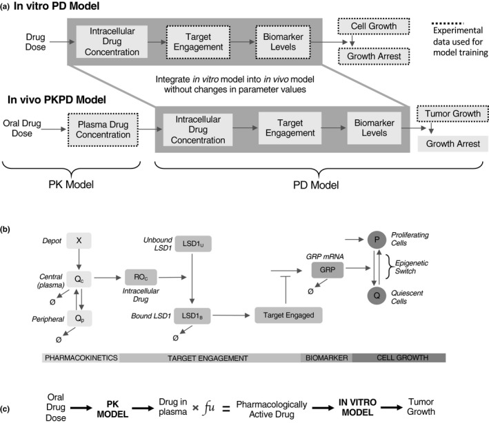
Model schematic overview and structure. (a) Flowcharts depicting generalized model overview for in vitro (above) and in vivo (below) models. The in vitro model quantitatively relates administered drug concentration to cell growth inhibition via target engagement and biomarker levels. The in vivo model is simply a composite of the in vitro model and an in vivo pharmacokinetics (PKs) model; the only adjustment to in vitro model parameters was a re‐estimation of cell growth in the tumor xenograft environment. Black dashed lines depict modules that were trained against experimental data; the rest were predicted by the model. (b) Kinetic scheme of model. The PK is modeled using a two‐compartment model, where a depot compartment (X) fuels a central compartment (Q c), which exchanges with a peripheral compartment (Q P). Cellular drug concentration (ROc) converts unbound LSD1 to bound LSD1, which can then be degraded. The ratio of bound to total LSD1 generated a percent target engaged quantity, which negatively regulates gastrin releasing peptide mRNA (GRP) levels. GRP levels then regulate an epigenetic switch between a proliferating (P) and quiescent (Q) cell population, provoking reversible cytostasis. (c) Methodological overview of scaling the in vitro model to the in vivo context. Drug in plasma was converted to drug in tumor cells scaled by experimentally determined fraction of unbound drug (fu, free drug in plasma). PD, pharmacodynamic.
In vivo pharmacokinetics
For in vivo PK, we used a two‐compartment PK model to characterize the plasma concentration time profile after oral administration of ORY‐1001 (Figure 1 b, far left). Following oral administration, ORY‐1001 undergoes first‐order absorption from a depot compartment (X) into the central compartment (Qc), which reversibly exchanges ORY‐1001 with a peripheral compartment (Qp) captured by the following equations:
| (1) |
| (2) |
| (3) |
| (4) |
| (5) |
The model was fit to multiple drug plasma concentration time courses performed in mice (Figure 4 a) using a gradient descent approach with multistart (see “Model parameters and parameter estimation” section on Parameter Estimation). This PK model was linked to the in vitro PD model via the unbound ORY‐1001 plasma concentration (fu in Figure 1 c) to yield the pharmacologically active drug (Figure 1 a). The pharmacologically active drug is linked to the PD model components, which are described below in greater detail.
Figure 4.
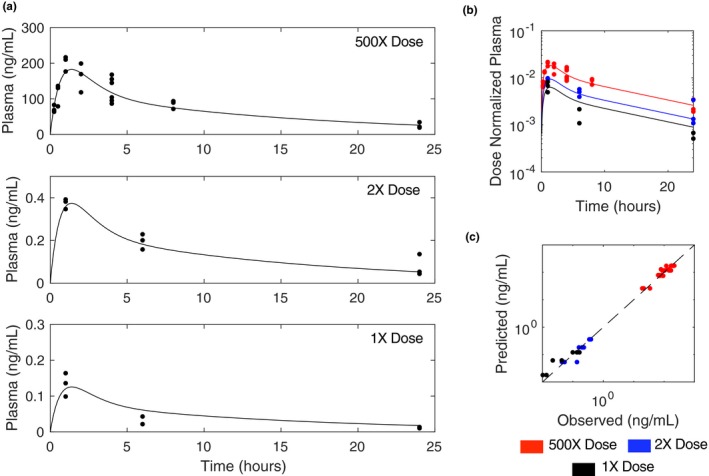
In vivo pharmacokinetic (PK) model. (a) Plasma profiles of orally administered ORY‐1001 in mice over 24 hours at various doses. (b) Dose normalized plasma PK profiles for each dose. (c) Predicted (simulations) vs. observed (experiments) plasma drug concentration.
Target engagement model
The model assumes that the drug effect is driven by the free drug concentration in the cell, which is assumed to be in equilibrium with the extracellular unbound drug concentration (Figure 1 c). It should be noted that this assumption is only applicable for small molecules and implies passive transport of the unbound and unionized molecules through membranes. It should be noted that this assumption is not valid if the drug of interest is a substrate of an active transporter, which will result in differences in the free concentration across membranes. Target engagement is modeled such that free intracellular drug (ROC) binds unbound LSD1 irreversibly,18 creating bound LSD1 (LSD1B; Eq. 7). LSD1B is subsequently degraded following Michaelis‐Menten kinetics. Thus, LSD1B is degraded faster as its concentration decreases. Here, we assumed negligible unbound drug decay (Eq. 6) as the compound was found to be stable in vitro over the experimental time scales. The ratio of bound to total LSD1 dictates percent target engaged and is captured by the following equations:
| (6) |
| (7) |
| (8) |
| (9) |
Biomarker model
The target engagement model is linked to the biomarker model assuming that the engaged target (TE) acts as negative regulator of GRP mRNA levels (Eq. 10; Figure 1 b) with a sigmoidal relationship. GRP mRNA follows first‐order degradation. We model kmax as being linearly dependent on the levels of GRP, essentially making GRP dependent on its own levels; that is, when it is lowly expressed, it becomes produced at a higher rate, and vice versa (Eqs. (10), (11), (12)). This was done in order to control the rebound dynamics of GRP after target engagement was released and introduces an additional level of GRP control beyond first‐order degradation. Biologically speaking, these types of feedback sensor systems are common in signaling, where the levels of a gene depends, either directly or indirectly, on its own levels, being dynamically tuned to optimize pathway function. The biomarker model is described by the following equations:
| (10) |
| (11) |
| (12) |
Cell growth dynamics model
Next, we assume that the GRP biomarker is a proxy for LSD1‐based control of tumor cell growth. Specifically, GRP expression controls a cellular state switch from proliferating (P) to quiescent (Q)—as GRP levels decrease, cells transition from P‐to‐Q, and vice versa (Figure 1 b) as described by the rates v PQ and v QP, depicted by the following equations:
| (13) |
| (14) |
| (15) |
| (16) |
| (17) |
| (18) |
| (19) |
| (20) |
Model parameters and parameter estimation
Initial conditions and model parameters are provided in Tables S1 and S2 , respectively. Analogous model optimization methods were applied to both the PK and PD models by first using a combination of manual approximation and lsqnonlin in Matlab (R2017b) to readily generate reasonable first‐pass estimates and then using a global estimation technique of gradient descent (fmincon in Matlab) with multistart.19 For the multistart optimizations, initial parameter estimates were obtained using latin hypercube sampling with a log normal distribution, with mean equal to our first‐pass parameter estimates and log10 SDs equal to 0.5 (log10 SD of 0.05 for Hill coefficients) without covariance between parameters. Upper and lower bounds were imposed to restrict parameters within physiologically relevant bounds (Table S2 ). This introduced up to ~ 100‐fold increase and decrease in parameters from their original values. A total of 2,122 parameter sets were obtained for the PD model (Figure S1 a) and 4,164 for the PK model (Figure S1 b). Each set has different parameter values and, therefore, different goodness of fit (sum of squared residual errors), and not all are guaranteed to be acceptable. Those fits in which the sum of squared residuals were no greater than twofold of those obtained from the first‐pass optimization were retained. For the PK model, 808 of 4,164 parameter sets met the criteria, whereas for the PD model 25 of 2,122 parameter sets did. (For PD model, parameter sets additionally had to predict in vivo efficacy as good as or better than our first‐pass parameter estimates.) The family of parameter sets meeting the threshold criteria were used to assess parameter variability, 95% confidence intervals, percent coefficient of variation, and lower and upper bounds for the PD (Figure S1 , Table S2 ) and PK (Figure S1 b, Table S2 ) models.
Compound stability
In vitro, ORY‐1001 was found to be metabolically stable in liver microsomes and hepatocytes across multiple species tested, with > 92% of drug being attributed to the parent drug as opposed to any metabolites. In vivo plasma, 70–90% of the exposure was parent compound as analyzed by mass spectrometry, the rest being minor metabolites.
Computation
The model was coded in MATLAB R2017b (code available as Supplemental Material). Simulations were run on a MacBook Pro with a 2.5 GHz Intel Core i5 processor and 16 GB of RAM. Ordinary differential equations were solved using the ode15s solver in MATLAB.
Target engagement experiments
NCI‐H510A cells were seeded and treated with ORY‐1001 for 24 hours. The compound was then washed off and the cells were kept in culture for three additional days in standard medium. Samples were collected at 24, 48, 72, and 96 hours post‐stimulus. Cells were treated with 0.6, 3, or 15 nM of drug. Percent target engagement was measured using an enzyme‐linked immunosorbent assay (ELISA)‐based technique that quantifies total and free LSD1, enabling the calculation of percent TE ().15, 20, 21, 22
Biomarker experiments
NCI‐H510A cells were seeded into 6 cm dishes and dosed with 0.1, 1, or 10 nM of compound or a vehicle control (H2O). Cells were harvested at 24, 96, or 168 hours post‐stimulus, washed once with phosphate‐buffered saline (PBS) then lysed in RLTplus buffer (Qiagen #79216) with 1% β‐mercaptoethanol. The mRNA was purified using a Maxwell beads‐based purification strategy, according to manufacturer’s protocols (Promega #AS1270), and the expression level of the GRP gene (UniGene: Hs.153444) was then determined using quantitative real‐time polymerase chain reaction (TaqMan RT‐PCR, Life Technologies #4392938) on a QS6 thermocycling instrument (AB). Relative quantification was determined using the ΔΔCt method, where a duplexed control (HPRT1, UniGene: Hs.412707) was used; expression changes were represented as a Log2 change from the reference sample (vehicle treatment at 24 hours).
Cell viability experiments
NCI‐H510A cells were seeded at an initial density of 8,000 cells per well in 96‐well plates. Viability assays were performed using the alamarBlue assay according to manufacturer’s protocols (Thermo #DAL1100). This fluorescent assay quantifies relative fluorescence units (RFU). To convert relative fluorescence units (RFU) to an absolute cell number quantity, we quantified RFUs of cells seeded at various densities ranging from < 1,000 to 16,000 cells per well and found a linear mapping (R 2 = 0.98; y = 6.14x–813.5), which we used to convert all subsequent RFU values.
In vivo PK experiments
The concentration of ORY‐1001 was determined using a liquid‐chromatography tandem mass spectrometry method in the plasma of tumor‐free mouse over a 24‐hour time period. The drug as well as spiked‐in internal standards were isolated from dipotassium (K2) EDTA mouse plasma from liquid‐liquid extraction with ammonium bicarbonate buffer and separated from other constituents of the sample by liquid‐chromatography tandem mass spectrometry. Detection was accomplished using turbo ion spray tandem mass spectrometry in positive ion selected reaction monitoring mode.
In vivo tumor xenograft experiments
NCI‐H510A cells were thawed in complete medium and grown for several weeks in 175 cm2 flasks to reach ~ 250 million cells. Cells were routinely subcultured once a week by gentle shaking in PBS. Cells growing in an exponential growth phase were harvested and counted before injection. Five million cells, in 100 μL of 1:1 Matrigel/PBS, were subcutaneously injected into female 7–8 week old athymic nude mice. After tumor growth reached 200‐300mm3, animals were distributed into different treatment groups. Tumors were monitored every other day or every 3 days for tumor volume (mm3).
Comparing nonlinear absorption to nonlinear clearance
We modeled nonlinear absorption as is depicted in the model equations above. To model nonlinear clearance we removed the bioavailability correction factor from Eq. 4 and instead replaced the clearance constant (k CL) from Eq. 2 with an equation of the form:
| (21) |
which introduces nonlinearity into the clearance term (Figure S3 ). lsqnonlin in MATLAB was used to find the best model fit to data. Final parameters were: = 0.15 (1/hour), = 2.02 (1/hour), = 0.05 (1/hour), = 80.3 (mL/kg), =27.2 (ng/mL), and = 68.7 (ng/(mL*hour)).
Global sensitivity analysis
We performed global sensitivity analysis as previously described by others.23 Parameter sets (30,000) were generated using latin hypercube sampling with log normal distribution, with means equal to the parameter values (Tables S1 and S2 ) and a log SD equal to 0.5 (SD equal to 0.05 for Hill coefficients). We assume no covariance between parameters. This introduced up to ~ 100‐fold increase and decrease in parameters from their original values. The in vitro model was evaluated at six drug doses (0, 0.01, 0.1, 1, 10, 100 nM) for each parameter set and three outputs were recorded: sum (across doses) of the areas under the curves for (i) target engagement (4 days), (ii) biomarker dynamics (7 days), and (iii) cell viability (10 days) over time. Next, a partial least squares regression (NIPALS algorithm) was conducted with parameter sets as predictor variables and each aforementioned output as observable variables (Figure S4 ). We used the regression model to predict model outputs. The relationship between actual values (x‐axis; regression model generated values) and predicted values (y‐axis; ODE model generated values) depicts a strong correlation, which speaks to the reliability of this method.
Results
Training of in vitro model
A comprehensive experimental protocol was used to cover a range of doses, time points, and dosing paradigms (continuous vs. pulsed) in order to characterize the preclinical PK/PD. We used six time course data sets (see Table 1): (i) target engagement, (ii) biomarker levels, (iii) drug‐free cell growth, (iv) drug‐treated cell viability, (v) in vivo drug‐free tumor growth, and (vi) in vivo drug PKs to train the in vitro model. Data for i‐v were collected exclusively from in vitro assays. Data for drug PK and xenograft tumor growth in the absence of drug were collected from in vivo assays (see Table 1 and dashed‐line rectangles in Figure 1 a). For the purposes of this study, we focused on the NCI‐H510A cell line, a well‐studied SCLC cell line known to be responsive to LSD1 inhibition.8
Target engagement was measured using an ELISA‐based technique that quantifies total and free LSD1, enabling the calculation of percent target engaged.15, 20, 21, 22 Measurements were collected at a range of doses (Figure 2 a, dots) at 24‐hour intervals over a 4‐day period. Cells were exposed to the drug for 24 hours followed by a removal and washout period for another 3 days. This pulse‐style experiment permitted the elucidation of decay kinetics in target engagement. Of some interest, target engagement seems to decay faster as drug concentration decreases. Although the precise mechanism underlying this is unknown, it could be mediated by nonlinearity in drug‐induced target turnover, and, thus, for the model, the degradation of bound LSD1 was cast as a saturable process (Eq. 2). The model was fit to these dose‐varying and time‐varying responses using nonlinear least squares parameter estimation procedures (see Methods).
Figure 2.
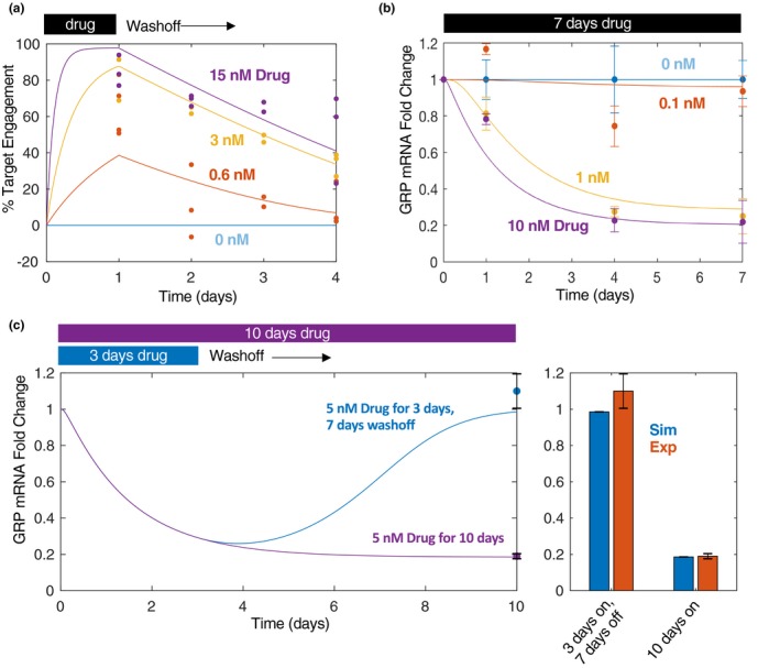
In vitro target engagement and biomarker dynamics. (a) ORY‐1001 was administered at different concentrations (at 0.6, 3, and 15 nM doses) for 24 hours, then the drug was washed off and fresh medium added. Percent target engaged was quantified using an enzyme‐linked immunosorbent assay‐based technology. Data were collected at the 24, 48, 72, and 96‐hour time points from the beginning of cell treatment. (b) ORY‐1001 was administered (at 0.1, 1, and 10 nM doses) for a total of 7 days and GRP mRNA levels were quantified using quantitative real‐time polymerase chain reaction at 1, 4, and 7 days post treatment. Three biological replicates were included per condition. (c) GRP mRNA levels quantified as before but in response to 5 nM pulsed (3 days on, 7 days off) or continuous (10 days on) treatment. Bar plot at 10 day time compares simulations with experiments (right). For all plots: lines = simulations; dots = experimental data. All experiments were performed in NCI‐H510A cells.
Target engagement was then linked to biomarker dynamics. GRP, a neuroendocrine gene whose levels are known to decrease in response to LSD1 inhibition in SCLC,8 was adopted as a biomarker using quantitative real‐time polymerase chain reaction (Figure 2 b). GRP mRNA levels were measured as a function of ORY‐1001 dose under both a continuous (Figure 2 b) and pulsed (Figure 2 c) exposure paradigm in order to assess drug effect durability. Following an initial 3‐day drug exposure, GRP levels returned to baseline levels by day 10 (Figure 2 c). The model was able to simultaneously capture the drug‐induced decrease in GRP levels as well as its return to baseline upon drug‐withdrawal.
Next, the relationships between mRNA GRP levels and cell growth were investigated by measuring cell growth over 10 days in the absence of drug, designed to capture the exponential phase of growth, and model parameters were estimated to fit these dynamics (specifically vP, Eqs. 4 and 10, inspired by prior work24; Figure 3 a). Next, end point dose‐response experiments were performed to capture the dose‐response relationship (Figure 3 b). These data were complimented with a “pulsed” dosing paradigm (Figure 3 c), in which drug was exposed for 3, 5, or 7 days followed by drug withdrawal for 7, 5, or 3 days, respectively. Again, the model was fit to simultaneously capture the continuous and pulsed dosing paradigms.
Figure 3.
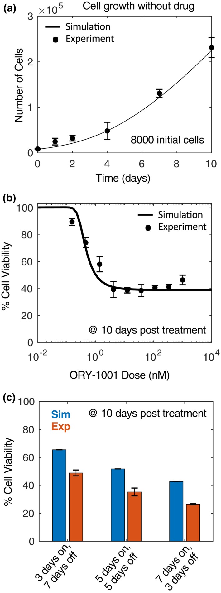
In vitro cell growth and viability. (a) Drug‐free cell growth was quantified at various time points (0, 1, 2, 4, 7, and 10 days). (b) Cell viability at various doses of ORY‐1001 at 10‐days post‐treatment (drug replenished at day 6). Lines = simulations; asterisks = experimental data. (c) Pulsed experiment comparing simulations (blue) with experiments (red). All assays performed at 10 days.
In vitro to in vivo scaling
The PK model was developed independently prior to linking it with the in vitro PD model. By fitting to three orally administered single‐dose ORY‐1001 time courses simultaneously, it was found that a two‐compartment model (Figure 1 b, far left) with nonlinear absorption best fit the data (Figure 4 a). Interestingly, the dose‐normalized plasma concentration time curves did not superimpose but were parallel shifted (Figure 4 b), indicative of nonlinear bioavailability. The nonlinear absorption model (modeled by estimating the fraction absorbed as a function of the total initial dose) provided a better fit to the experimental data than a nonlinear clearance model (modeled as a function of the drug plasma concentration, Figures 4 c, S1 , and S3 ).
Next, to link the two‐comparment PK model of ORY‐1001 to the in vitro PD, we assumed intracellular drug concentration to be equal to the unbound plasma concentration based on the experimentally determined value of fu = 0.75 in mice. This assumption is supported by the fact that there was no evidence for transporter involvement to the distribution or elimination of ORY‐1001 based on nonclinical studies (data‐on‐file, not shown). Finally, to convert the cell growth metric from number of cells (in vitro) to tumor size in units of mm3 (in vivo), cell growth parameters, k P and k 50P (Eq. 15), were re‐estimated enabling a model fit to drug‐free growth of NCI‐H510A cells in mouse xenografts. This was also done to capture the slower growth of cells in the in vivo tumor environment compared with the cell culture setting. No additional changes were made to generate the final in vivo PK/PD model. All of the remaining parameters—including those governing drug control over target engagement, target engagement control over biomarker levels, and biomarker‐driven epigenetic switching—remained exactly as they were in the in vitro model (see Table S2 for parameter values).
In vivo model predictions and validation
The in vivo PK/PD model of ORY‐1001 was used to predict drug plasma concentration, drug tumor concentration, percent TE, and GRP mRNA levels across a time course of 30 to 35 days under different multiple‐dosing scenarios (Figure 5 a). In addition, tumor growth dynamics were also predicted under the same dosing scenarios (Figure 5 b, blue lines). Mice bearing NCI‐H510A xenografts were monitored for tumor size (mm3) over these dosing scenarios following subcutaneous cell implantation and compared with simulated predictions (Figure 5 b). Remarkably, the in vivo model predictions agreed well with the in vivo measurements, based on comparing actual to simulated tumor volumes for all time points (Figure 5 c) and also by assessing the ratio between actual and predicted area under the tumor growth inhibition curve (Figure 5 d). This is noteworthy given that no changes were made to the parameter values underlying drug sensitivity, but only to cell growth dynamics (parameter k P), as described above, based on data without drug treatment. In addition, a global sensitivity analysis further supported that cell viability outcomes were highly sensitive to cell growth parameters, k P and K 50P (Figure S4 ). The model‐predicted drug plasma/tumor concentration, target engagement, and GRP mRNA dynamics in the tumor, could hold relevance in defining expected preclinical biomarker levels that dictate drug efficacy.
Figure 5.
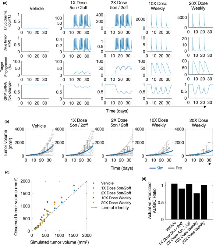
In vivo drug efficacy predictions. (a) Various dosing regimens simulated and drug plasma concentration, drug tumor concentration, target engagement, and gastrin releasing peptide (GRP) mRNA levels are shown. (b) Simulated tumor volume time course for various dosing regimens (blue lines) compared with experimental measurements. Asterisks, experimental mean; grey lines, individual mice trajectories. (c) Scatter plot of simulated vs. actual tumor volumes across time course as in (b). Each dot represents a single time point for which an experimental comparison exists. (d) Ratio between the area under the tumor growth inhibition curve (AUGIC) between the simulated (predicted) and experimental (actual) data for each dosing regimen. A ratio equal to one indicates an exact match.
Discussion
Here, we built a semimechanistic PK/PD model to describe the efficacy of a small‐molecule inhibitor, ORY‐1001, of an epigenetic regulator implicated in cancer, LSD1. We successfully incorporated a model trained almost exclusively on in vitro data—with the exception of the intrinsic drug‐free cell growth parameter (k P)—with a PK model to predict in vivo antitumor efficacy in mouse xenografts of SCLC. Three major types of measurements informed key PD events: (i) cellular drug concentration, (ii) percent TE, (iii) biomarker dynamics, and (iv) cell growth dynamics. This permitted the capture of both the acute (target engagement) as well as the more prolonged (biomarker changes) effects of the drug. Furthermore, the incorporation of pulsed as well as continuous dosing paradigms in vitro enabled the model to capture the durability of drug effect. This is likely to be generally important when translating to the in vivo setting as drug concentration is not static but is rather dynamic with dependencies relating to drug dose, dosing regimen, clearance rate, and absorption kinetics. This is of particular relevance for drugs affecting epigenetic factors, like LSD1 and/or irreversible inhibitors such as ORY‐1001, as their effects may be more durable than other treatment modalities. Moreover, focusing on in vitro data sets permitted more time points and doses, in a more controlled and reproducible setting, compared with if all experiments had been performed in vivo.
One of the major differences between in vitro and in vivo systems could be the potential formation of major active metabolites, which can contribute to the overall drug effect. When predicting in vivo efficacy from in vitro data, the model should account for the formation of these major active metabolites as well as potential differences with regard to drug potency and drug disposition between the parent drug and any metabolites. Here, the potential contribution of major active metabolites to in vivo activities was not taken into account in the model because (i) ORY‐1001 was found to be stable in vitro in liver microsomes and hepatocytes from humans, mice, rats, and dogs, and (ii) in vivo absorption, distribution, metabolism, and excretion study in rats dosed of [14C]‐labeled ORY‐0001 showed the major circulating drug‐related component was the parent form (data‐on‐file, not shown).
The proposed model assumes that the pharmacological active concentration is the free intracellular drug concentration, which, under steady‐state conditions, is the same as the free plasma concentration. It should be noted that this assumption is only applicable for small molecules and implies passive transport of the unbound and unionized molecules through membranes. It is not valid if the drug of interest is a substrate of an active transporter or undergoes carrier‐mediated membrane transport, which will produce differences in the free concentrations across the membranes. However, in the present study, there was no evidence for transporter involvement to ORY‐1001’s distribution or elimination based on nonclinical studies (data‐on‐file, not shown).
Limitations of this study include the use of a single biomarker, GRP, which may not be relevant for different cells or patients. An improvement would be to incorporate additional biomarkers in conjunction with a mechanistic understanding of how they regulate one another, so as to merge mechanism of action with drug effectiveness in a more comprehensive fashion. Furthermore, the current study is limited due to the use of a single cell line. The extrapolation of this model to other cell lines, especially cell lines that are insensitive to LSD1 inhibition, will be important to determine the model’s general applicability. Last, future versions of this model should be scaled to humans, harnessing tumor growth and biomarker data from clinical trials.
In conclusion, the model herein, trained primarily using in vitro cell kinetic data sets, is predictive of in vivo drug efficacy, whereas only requiring two in vivo measurements: PK and drug‐free tumor growth dynamics. This suggests that in vitro dose responsiveness can be predictive in vivo, although we recommend more cell lines be studied in this way to assess the robustness of this approach. Furthermore, this modeling effort introduced an epigenetic switch mechanism through the use of a key biomarker for LSD1 inhibition that may constitute a valuable approach for modeling other epigenetic modifiers. In general, pairing in‐depth in vitro research with mathematical modeling may enable the reduction of animal usage, the ability to optimize experimental strategies, to comprehensively explore drug‐response relationships, and to probe mechanisms underlying drug effectiveness in quantitative terms.
Funding
This work was funded by R01GM104184 and sponsored by Oryzon Genomics and F. Hoffmann‐La Roche Ltd.
Conflict of Interest
M.B., L.J.Y., F.M., S.K.S., and A.C.W. are current or former employees of F. Hoffmann‐La Roche Ltd. S.L. was employed by Oryzon Genomics while performing this work. All other authors declared no competing interests for this work.
Author Contributions
M.B., L.J.Y., F.M., J.M.G., M.R.B., and A.C.W. wrote the manuscript. A.C.W., L.J.Y., M.R.B., J.M.G., M.B., F.M., S.L., and S.K.S. designed the research. M.B., S.L., S.K.S., and A.C.W. performed the research. M.B., S.L., L.J.Y., A.C.W., and M.R.B. analyzed the data.
Supporting information
Figure S1. Parameter estimation results. (a) For PD (in vitro) model, a total of 2,122 parameter sets were run using a multi‐start gradient descent approach. Of those, 25 parameter sets possessed acceptable error when comparing simulations to experiments and also predicted in vivo tumor growth with good accuracy (see Methods). Here, we depict the variability for each parameter (blue dots) within its upper and lower bounds (red lines). (b) Similar to in (a), 4,164 parameter sets were run using a multi‐start gradient descent approach estimate parameters for the PK model only. Of those, 808 sets possessed acceptable error. Here, we depict the variability for each of the PK parameters (blue dots) within their upper and lower bounds (red lines). White circles: median.
Figure S2. Model predictions of individual variability of in vivo drug response. (a) Individual mice treated with the indicated dosing regimens (top, grey) are compared with model simulations (bottom, blue). Modification of the cell growth constant to capture the fastest (k P = 0.0048) and slowest (k P = 0.0022) growing tumors (dotted blue lines), above and below the original model simulations (solid blue line, k P = 0.0037), respectively, recapitulates some (i.e. range) of the variability between mice. (b) Experimental mean (black dot), standard deviations (grey boxes), and range (black line) for experiments shown on left. On right, analogous simulations depict primary model fit to mean experimental data (black dot) and range between the minimum and maximum model simulations from (a), bottom.
Figure S3. Non‐linear absorption vs. non‐linear clearance. (a) Dose normalized plasma drug concentrations are plotted for each dose. A model depicting non‐linear absorption (left) is compared with one depicting non‐linear clearance (right). (b) Predicted (simulated) vs. observed (experimental) plot for each dose. In general, a model depicting non‐linear absorption provides a better fit to the data.
Figure S4. Global sensitivity analysis. (a) Parameter sensitivity for target engagement (blue), biomarker levels (red), and cell viability (yellow). 30,000 randomly sampled parameter sets were simulated at various doses and area under model curves were calculated, one for each model output. A partial least squares regression (NIPALS algorithm) was used to calculated regression coefficients linking predictor variables (parameter sets) to model outputs. (b) Actual vs. regression‐predicted values using the regression model. The strong correlation speaks to the reliability of this method.
Table S1. Model initial conditions.
Table S2. Model parameters.
Acknowledgments
The authors thank Roche and Oryzon LSD1 teams and management for their support and helpful discussions.
Contributor Information
Marc R. Birtwistle, Email: mbirtwi@clemson.edu.
Antje‐Christine Walz, Email: antje-christine.walz@roche.com.
References
- 1. Benson, N. , Cucurull‐Sanchez, L. , Demin, O. , Smirnov, S. & Van Der Graaf, P.V. Reducing systems biology to practice in pharmaceutical company research: selected case studies. Adv. Exp. Med. Biol. 736, 607–615 (2012). [DOI] [PubMed] [Google Scholar]
- 2. van der Greef, J. & McBurney, R.N. Rescuing drug discovery: in vivo systems pathology and systems pharmacology. Nat. Rev. Drug Discov. 4, 961–967 (2005). [DOI] [PubMed] [Google Scholar]
- 3. Bouhaddou, M. et al. A mechanistic pan‐cancer pathway model informed by multi‐omics data interprets stochastic cell fate responses to drugs and mitogens. PLoS Comput. Biol. 14, e1005985 (2018). [DOI] [PMC free article] [PubMed] [Google Scholar]
- 4. Higgins, B. et al. Preclinical optimization of MDM2 antagonist scheduling for cancer treatment by using a model‐based approach. Clin. Cancer Res. 20, 3742–3752 (2014). [DOI] [PubMed] [Google Scholar]
- 5. van der Graaf, P.H. & Benson, N. Systems pharmacology: bridging systems biology and pharmacokinetics‐pharmacodynamics (PKPD) in drug discovery and development. Pharm. Res. 28, 1460–1464 (2011). [DOI] [PubMed] [Google Scholar]
- 6. Checkley, S et al. Bridging the gap between in vitro and in vivo: dose and schedule predictions for the ATR inhibitor AZD6738. Sci. Rep. 5, 13545 (2015). [DOI] [PMC free article] [PubMed] [Google Scholar]
- 7. Maes, T. et al. ORY‐1001, a potent and selective covalent KDM1A inhibitor, for the treatment of acute leukemia. Cancer Cell 33, 495–511.e12 (2018). [DOI] [PubMed] [Google Scholar]
- 8. Mohammad, H.P. et al. A DNA hypomethylation signature predicts antitumor activity of LSD1 inhibitors in SCLC. Cancer Cell 28, 57–69 (2015). [DOI] [PubMed] [Google Scholar]
- 9. Crabtree, J.S. & Miele, L. Neuroendocrine tumors: current therapies, notch signaling, and cancer stem cells. J. Cancer Metastasis Treat. 2, 279 (2016). [Google Scholar]
- 10. Lamballe, F. et al. Coordination of signalling networks and tumorigenic properties by ABL in glioblastoma cells. Oncotarget 7, 74747–74767 (2015). [DOI] [PMC free article] [PubMed] [Google Scholar]
- 11. Zhao, ZK et al. Overexpression of lysine specific demethylase 1 predicts worse prognosis in primary hepatocellular carcinoma patients. World J. Gastroenterol. 18, 6651–6656 (2012). [DOI] [PMC free article] [PubMed] [Google Scholar]
- 12. Yu, Y. et al. High expression of lysine‐specific demethylase 1 correlates with poor prognosis of patients with esophageal squamous cell carcinoma. Biochem. Biophys. Res. Commun. 437, 192–198 (2013). [DOI] [PubMed] [Google Scholar]
- 13. Lv, T. et al. Over‐expression of LSD1 promotes proliferation, migration and invasion in non‐small cell lung cancer. PLoS One 7, e35065 (2012). [DOI] [PMC free article] [PubMed] [Google Scholar]
- 14. Jie, D et al. Positive expression of LSD1 and negative expression of E‐cadherin correlate with metastasis and poor prognosis of colon cancer. Dig. Dis. Sci. 58, 1581–1589 (2013). [DOI] [PubMed] [Google Scholar]
- 15. Maes, T. et al. ORY‐1001, a potent and selective covalent KDM1A inhibitor, for the treatment of acute leukemia. Cancer Cell 12, 495–511 (2018). [DOI] [PubMed] [Google Scholar]
- 16. Adamo, A et al. LSD1 regulates the balance between self‐renewal and differentiation in human embryonic stem cells. Nat. Cell Biol. 13, 652–661 (2011). [DOI] [PubMed] [Google Scholar]
- 17. Harris, W.J. et al. The histone demethylase KDM1A sustains the oncogenic potential of MLL‐AF9 leukemia stem cells. Cancer Cell 21, 473–487 (2012). [DOI] [PubMed] [Google Scholar]
- 18. Binda, C. et al. Biochemical, structural, and biological evaluation of tranylcypromine derivatives as inhibitors of histone demethylases LSD1 and LSD2. J. Am. Chem. Soc. 132, 6827–6833 (2010). [DOI] [PubMed] [Google Scholar]
- 19. Frohlich, F. , Kaltenbacher, B. , Theis, F.J. & Hasenauer, J. Scalable parameter estimation for genome‐scale biochemical reaction networks. PLoS Comput. Biol. 23, e1005331 (2017). [DOI] [PMC free article] [PubMed] [Google Scholar]
- 20. Gonzales, E.C. , Maes, T. , Crusat, C.M. & Munoz, A.O . Methods to determine kdm1a target engagement and chemoprobes useful therefor. Patent WO2017158136, Oryzon Genomics. (2017).
- 21. Mascaró, C. , Ruiz, R.R. & Maes, T. Direct measurement of KDM1A target engagement using chemoprobe‐based immunoassays. J. Vis. Exp. 148, e59390 (2019). [DOI] [PubMed] [Google Scholar]
- 22. Mascaró, C. et al. Chemoprobe‐based assays of histone lysine demethylase 1A target occupation enable in vivo pharmacokinetics and pharmacodynamics studies of KDM1A inhibitors. J. Biol. Chem. 17, 8311–8322 (2019). [DOI] [PMC free article] [PubMed] [Google Scholar]
- 23. Sobie, E.A. Parameter sensitivity analysis in electrophysiological models using multivariable regression. Biophys. J. 96, 1264–1274 (2009). [DOI] [PMC free article] [PubMed] [Google Scholar]
- 24. Mould, D.R. , Walz, A.C. , Lave, T. , Gibbs, J.P. & Frame, B. Developing exposure/response models for anticancer drug treatment: Special considerations. CPT Pharmacometrics Syst. Pharmacol. 4, 12–27 (2015). [DOI] [PMC free article] [PubMed] [Google Scholar]
Associated Data
This section collects any data citations, data availability statements, or supplementary materials included in this article.
Supplementary Materials
Figure S1. Parameter estimation results. (a) For PD (in vitro) model, a total of 2,122 parameter sets were run using a multi‐start gradient descent approach. Of those, 25 parameter sets possessed acceptable error when comparing simulations to experiments and also predicted in vivo tumor growth with good accuracy (see Methods). Here, we depict the variability for each parameter (blue dots) within its upper and lower bounds (red lines). (b) Similar to in (a), 4,164 parameter sets were run using a multi‐start gradient descent approach estimate parameters for the PK model only. Of those, 808 sets possessed acceptable error. Here, we depict the variability for each of the PK parameters (blue dots) within their upper and lower bounds (red lines). White circles: median.
Figure S2. Model predictions of individual variability of in vivo drug response. (a) Individual mice treated with the indicated dosing regimens (top, grey) are compared with model simulations (bottom, blue). Modification of the cell growth constant to capture the fastest (k P = 0.0048) and slowest (k P = 0.0022) growing tumors (dotted blue lines), above and below the original model simulations (solid blue line, k P = 0.0037), respectively, recapitulates some (i.e. range) of the variability between mice. (b) Experimental mean (black dot), standard deviations (grey boxes), and range (black line) for experiments shown on left. On right, analogous simulations depict primary model fit to mean experimental data (black dot) and range between the minimum and maximum model simulations from (a), bottom.
Figure S3. Non‐linear absorption vs. non‐linear clearance. (a) Dose normalized plasma drug concentrations are plotted for each dose. A model depicting non‐linear absorption (left) is compared with one depicting non‐linear clearance (right). (b) Predicted (simulated) vs. observed (experimental) plot for each dose. In general, a model depicting non‐linear absorption provides a better fit to the data.
Figure S4. Global sensitivity analysis. (a) Parameter sensitivity for target engagement (blue), biomarker levels (red), and cell viability (yellow). 30,000 randomly sampled parameter sets were simulated at various doses and area under model curves were calculated, one for each model output. A partial least squares regression (NIPALS algorithm) was used to calculated regression coefficients linking predictor variables (parameter sets) to model outputs. (b) Actual vs. regression‐predicted values using the regression model. The strong correlation speaks to the reliability of this method.
Table S1. Model initial conditions.
Table S2. Model parameters.