Fig. 4.
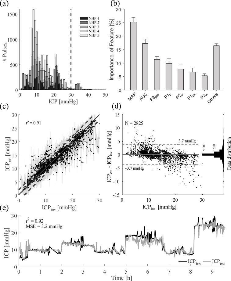
Results of the regression forest machine learning approach. (a) shows the distribution of the available data. The dashed line marks the maximum ICP level that was fitted for at 30 mmHg. (b) shows the distribution of features used in the regression forest as a percentage of all chosen features in all decision criteria generated. The standard deviation across individual trees is shown as error bars. Nomenclature is according to Table 1. (c) shows the performance of the regression forest by plotting estimated ICP (ICPest) over invasively measured ground truth (ICPinv). The solid line shows the ideal fit, while the dashed lines mark an area of 2 mmHg around the ideal fit. The shaded area shows the confidence interval. (d) graphs the difference between ICPest and ICPinv over ICPinv in a Bland-Altman plot. The dashed lines span a region of 95% of the distribution, corresponding to a standard deviation of 1.96. The histogram on the right of this graph shows the distribution of data points in number of samples. (e) shows a continuous estimate of ICP for NHP 3. The gray line shows the estimated ICP, and the black line the invasively measured ICP. An r2 = 0.92 and a mean squared error MSE = 3.2 mmHg were achieved.

