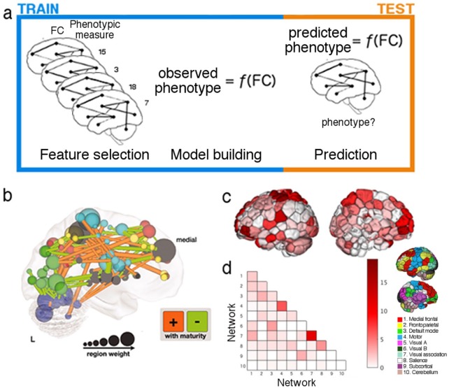
Figure 8.

Predictive modeling follows a standard framework, and models are most effectively trained and summarized by using combinations of region- and connection-based measures. (a) Predictive modeling involves three general steps: feature selection, in which a subset of all features is selected from the training data; model building, in which those features are submitted to an algorithm that fits them to a set of observed measures; and prediction, in which feature selection is performed on previously unseen test data, and resulting features are submitted to the models to yield a prediction of the measure of interest (indicated in the figure by “phenotype?”). This process is repeated iteratively, with different divisions of data into training and test sets on each iteration. (b) While projecting connection-based features used for prediction onto the brain can become difficult to interpret due to the sheer number of features, using both region- (e.g., region weight [as indicated by node size] or network membership [as indicated by node color]) and connection-based measures (as indicated by lines between nodes) can aid model summarization and interpretation. Alternative visualization methods focus on one measure at a time to aid interpretation. In (c), nodes are colored according to their binary degree (total number of connections incident to that node in the given model), while in (d), each connection in the given model is assigned to a pair of networks (see inset for a visualization of the 10 networks used in this example). Together, such depictions provide complementary insights into the locations of overrepresented regions (c) and connections (d), while avoiding the difficulty of interpreting individual connections or model weights. Adapted with permission from: “b”: Dosenbach and others (2010) and “c-d”: Greene and others (2018).