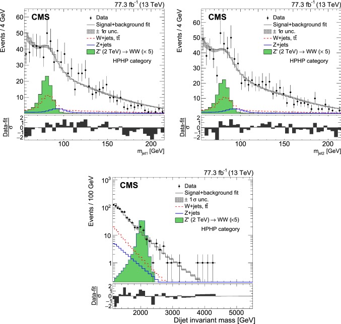
Fig. 10.

For the HPHP category: comparison between the signal+background fit and the data distributions of $m_{\mathrm{jet}1}$ (upper left), $m_{\mathrm{jet}2}$ (upper right), and $m_{\mathrm{jj}}$ (lower). The background shape uncertainty is shown as a gray shaded band, and the statistical uncertainties of the data are shown as vertical bars. An example of a signal distribution is overlaid, where the number of expected events is scaled by a factor of 5. Shown below each mass plot is the corresponding pull distribution $(\text{Data-fit})/\sigma$, where $\sigma =\sqrt{{\sigma }_{\mathrm{data}}^2-{\sigma }_{\mathrm{fit}}^2}$ for each bin to ensure a Gaussian pull-distribution, as defined in Ref. [83]