. 2020 Mar 13;9:e51972. doi: 10.7554/eLife.51972

Figure 4. Neocortex tends to sequentially activate from medial to more lateral regions around SWRs.

(A) (i) Demonstration of how peri-SWR neocortical activation peak time (tp) was quantified. The mean peri-SWR neocortical activity trace was generated for each region (blue trace) and the timestamp of the peak was defined as tp. (ii) Peri-SWR activation peak timestamp (tp) relative to SWR centers (0s-time) across neocortical regions sorted in ascending order. Each line graph represents one animal. tp values were not detected in some regions and in some animals (three data points in total), mainly because there was not a strong activation in those regions. Such missing data points were filled by average of available data points in the same region and in other animals (repeated measure ANOVA: F8,104 = 8.357195, p<0.0001; post-hoc test for linear trend: slope = 0.003252024 s/region, p<0.0001). (iii) Spatial map of peri-SWR activation peak time across all animals (n = 14) indicating a medial-to-lateral direction of activation. The red area was not included in this analysis because it was not activated strong enough to yield a reliable result. (B) (i) Circular distributions represent the direction of propagating waves of activity in three distinct neocortical regions at hippocampal SWR (blue distribution) and at random timestamps generated by shuffling inter-SWR time intervals (red distribution). 180–0 and 90–270 degrees represent the medio-lateral and antero-posterior axes, respectively. P-values come from Kuiper two-sample test. (ii) Schematic of propagation directions measured at SWR timestamps in three neocortical regions located in the medial neocortex. This figure has two figure supplement.

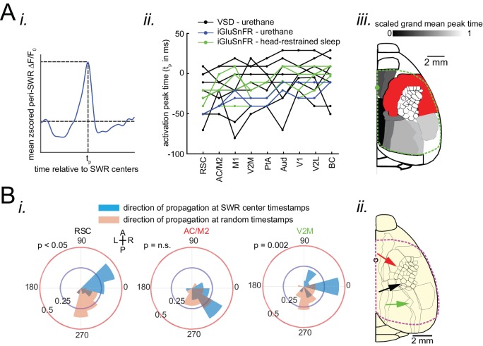
Figure 4.

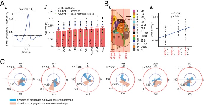
Figure 4—figure supplement 1. Neocortex tends to activate sequentially from medial to more lateral regions around SWRs.

Figure 4—figure supplement 1.

(A) (i) Demonstration of how peri-SWR neocortical activation rise time was measured. Rise time was calculated as the time which takes for the signal to reach 90% of the peak value starting from 10%. (ii) Summary of the mean peri-SWR activation rise time across neocortical regions from n = 12–14 mice imaged during states of urethane anesthesia (blue and black dots) and head-restrained sleep (green dots). There is no significant difference in activation rise time across neocortical regions meaning that all imaged neocortical regions activate at the same rate. It suggests that activation peak time can reflect the activation time of a given region. The bar graphs are mean ± SEM. (B) Schematic representation of vertical stripes splitting the recorded neocortical regions from medial to lateral into four groups. (ii) There is a significant correlation (r = 0.429, p<0.01, two-sided t-test) between stripe number and peak activation timestamp (tp) indicating that the more lateral regions activate later than medial ones relative to hippocampal SWRs. Dots represent the average tp across regions in each stripe and for each animal. (C) Circular distributions represent the direction of neocortical propagating waves of activation in a given region at hippocampal SWR timestamps (blue distribution) and at random timestamps generated by shuffling inter-SWR time intervals (red distribution). 180–0 degrees represent the medio-lateral and 90–270 degrees represent the antero-posterior axes (p-values are calculated based on Kuiper two-sample test).
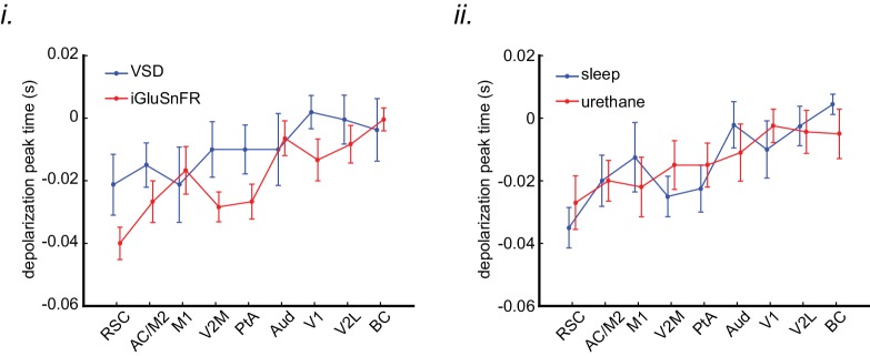
Figure 4—figure supplement 2. The order of sequential activation across neocortical regions around SWRs is similar under sleep/urethane anesthesia and VSD/iGluSnFR imaging conditions.

Figure 4—figure supplement 2.

The peak time of mean peri-SWR activation across neocortical regions is displayed for VSD versus iGluSnFR (i) and sleep versus urethane anesthesia (ii) conditions. The regions on the horizontal axes are sorted in an increasing order based on the average of all animals (n = 14) in each region. The linear trend in all the four conditions are statistically significant (repeated measure ANOVA follow-up test for linear trend; VSD: slope = 0.002665 s/region, iGluSnFR: slope = 0.004034 s/region, sleep: slope = 0.003968 s/region, and urethane: slope = 0.002966 s/region; All the p-values are less than 0.0001). Error bars represent standard errors.