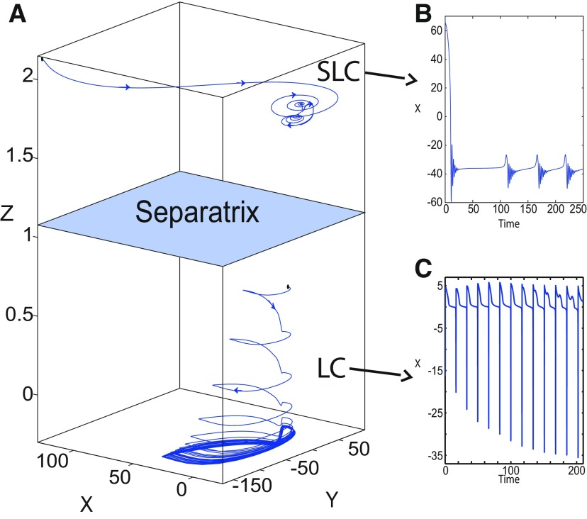
Figure 24.

A, Coexistence of SLC and RSE. The simulations are performed without noise. SLC and a stable LC coexist for m = −2 and $x_0=0$ ($I_{ex{t}_2}=0$). The equilibrium point is an unstable focus. The arrows indicate the direction of trajectories. For easier visualization, we plot generalized coordinates (X, Y, Z) corresponding to ($-60x_1+x_2,\hspace{0.17em}60y_1,\hspace{0.17em}z-0.5$) for SLC (top) and to ($-0.5x_1+x_2,\hspace{0.17em}0.1y_1,\hspace{0.17em}z+1.7$) for LC (bottom). LC is characteristic of RSE. B, C, Time series of SLC (B) and LC (C). Parameter settings correspond to region II in Figure 34 and to region 2 in Figure 35. A, Top, I.C = [−1.15 −5 2.9 0 0 0.01], $T_s=[0:0.01:250]$, and r  =  0.007. A, Bottom, I.C = [10 −5 −1 0 0 0.01], T_s = [0 500], and r  =  0.002. The coexistence of LC, S, and SLC can be found in area III [Fig. 12B].