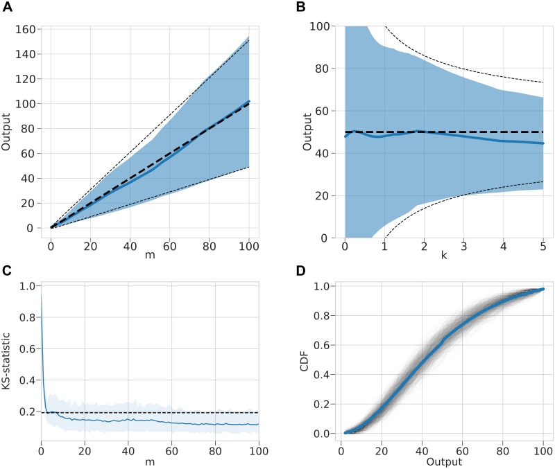
Fig 2. Gamma-MDN output emulating a negative binomial model.
(A) For fixed shape parameter k = 2.5, the distribution of output from MDN is shown in blue (mean = solid line, variance = shaded region), the theoretical values are shown as a black dashed line (mean = bold line, variance = normal line). (B) For fixed mean parameter m = 50, the distribution of output from MDN over a range of k values is shown in blue (mean = solid line, variance = shaded region), the theoretical values are shown as a black dashed line (mean = bold line, variance = normal line). (C) Corresponding two-sample K–S statistic where sample of 100 points are drawn from a negative binomial and the MDN over a range of m values. 100 replicates are used to estimate a mean K–S statistic and a 95% range. The dashed line represents significance at α = 0.05, with values less than this indicating that the two samples do not differ significantly. (D) Example empirical CDFs drawn from 100 samples of MDN with inputs m = 50 and k = 2.5. 1,000 empirical CDFs are shown as black transparent lines and true CDF is shown as a blue solid line.

